Swing-Up Control of Pendulum Using Multistage Nonlinear MPC with Nonlinear Grey-Box Model

This example uses a multistage nonlinear model predictive controller to swing-up and balance an inverted pendulum on a cart. The nonlinear plant that you use to design the MPC controller is a grey-box model in which three parameters are known and the other two parameters are estimated from input-output data.

Estimate Pendulum and Cart Grey-Box Model

The nonlinear plant is the pendulum and cart assembly system as shown in the figure.

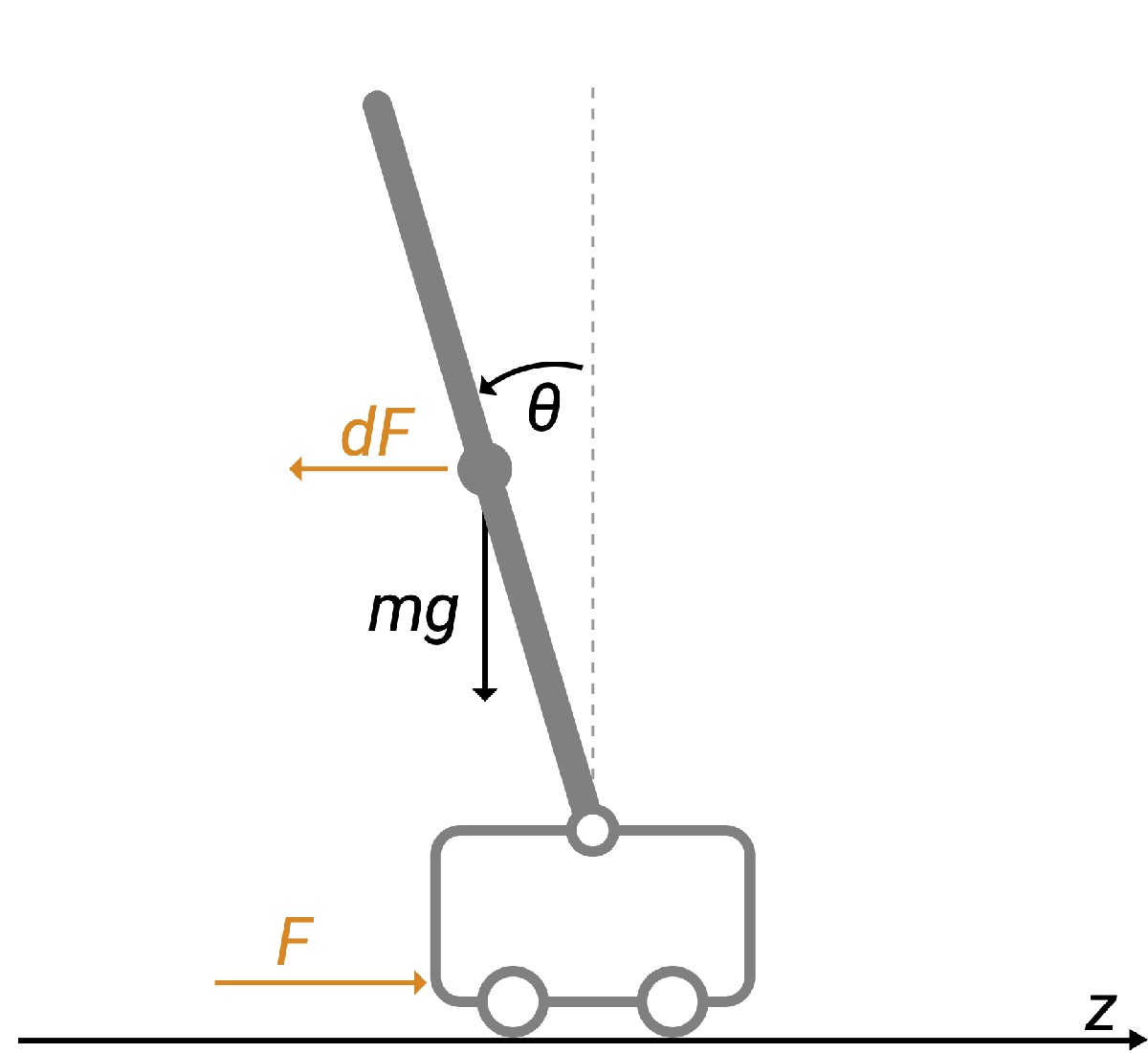
The plant model consists of four states: cart position, cart velocity, pendulum angle, and pendulum angular velocity. The control variable is the force (F) with an impulsive disturbance (dF) acting on the cart. The measured outputs are the cart position (z) and pendulum angle ($\theta$).

The example Swing-Up Control of Pendulum Using Nonlinear Model Predictive Control, also uses this model, illustrating it with more detail. In that example, you use the model state transition and output functions directly for nonlinear MPC design, instead of a grey-box model. For a more thorough explanation of the model conventions and how to derive the underlying system equations, see Derive Equations of Motion and Simulate Cart-Pole System (Symbolic Math Toolbox).

To estimate the model, load the available input-output data from the MAT file. The data consists of a uniformly sampled data set with 4001 samples in the variables u and y with a sample time of 0.01 second. The input (u) is the force applied on the cart, which is a periodic sinusoidal signal. The corresponding output (y) is a vector containing the cart position and pendulum angle.

load("pendulum_cart_data.mat")

Create an iddata (System Identification Toolbox) object to represent and store the data. For more information, see Representing Time- and Frequency-Domain Data Using iddata Objects (System Identification Toolbox).

z = iddata(y,u,0.01,Name="Pendulum Cart Data");

Assign names and units to the stored signals.

z.InputName = {'Angle'};
z.InputUnit = {'rad'};
z.OutputName = {'x';         ... % Position of the Cart
                'theta'     ... % Angle of the Pendulum
                };
z.OutputUnit = {'m'; 'rad'};
z.Tstart =  0;
z.TimeUnit = 's';

The system has five parameters: mass of the cart (M), mass of the pendulum (m), gravitational acceleration (g), length of the pendulum (l), and the damping coefficient (Kd). Three of these parameters (m, g, and l) are assumed to be known. To create the idnlgrey (System Identification Toolbox) object, first, organize the parameter details into a structure. The structure contains parameter names, units, initial values, limits, and a logical variable indicating whether the true parameter value is known.

Parameters = struct( ...
    ... % Names.
    "Name", ...
    {   "Mass of the Cart"               ...  % M
        "Mass of the Pendulum"           ...  % m
        "Gravitational Acceleration"     ...  % g
        "Length of the Pendulum"         ...  % l
        "Damping Coefficient"            ...  % Kd
    }, ...
    ... % Units
    "Unit", ...
    {"Kg", "Kg", "m/s^2", "m", "Ns/m"}, ...
    ... % Values
    "Value", ...
    {0.4, 1, 9.81, 0.5, 6}, ...
    ... % Constraints.
    "Minimum", {-Inf -Inf -Inf -Inf -Inf}, ...
    "Maximum", {Inf Inf Inf Inf Inf}, ...
    ... % M and Kd are unknown.
    "Fixed", {false true true true false});       

The provided swingup_m.m function implements the system dynamics of the model.

type("swingup_m.m")

function [dxdt, y] = swingup_m( ...
    ~, x, u, M, m, g, l, Kd, varargin)
%% Continuous-time nonlinear dynamic model 
% of a pendulum on a cart
%
% 4 states (x): 
%   cart position (z)
%   cart velocity (z_dot): positive right
%   angle (theta): 0 at upright position
%   angular velocity (theta_dot): 
%                       counterclockwise positive
% 
% 1 inputs: (u)
%   force (F): when positive, 
%                       force pushes cart to right 
%
% Copyright 2024 The MathWorks, Inc.


%% Obtain x, u and y

% x
z_dot = x(2);
theta = x(3);
theta_dot = x(4);

% u
F = u;

%% Compute dxdt
dxdt = [
    
    z_dot;...

    (   F - Kd*z_dot ...
        - m*l*theta_dot^2*sin(theta) ...
        + m*g*sin(theta)*cos(theta)...
    )/(M + m*sin(theta)^2); ...

    theta_dot; ...

    (  g*sin(theta) + ...
       (F - Kd*z_dot - m*l*theta_dot^2*sin(theta))*...
       cos(theta)/(M + m) ...
    )/(l - m*l*cos(theta)^2/(M + m))

    ];

% y
y = [x(1);x(3)];

Use the model file, along with the order, parameters, and initial states data, to create an idnlgrey object that represents the nonlinear grey-box model of the system.

Filename = "swingup_m";             % Model ODE file
Order = [2 1 4];                    % Model orders [ny nu nx]
InitialStates = [0; 0; -pi; 0];     % Initial states values
Ts = 0;                             % Continuous-time system

% Create idnlgrey object.
nlgr = idnlgrey(Filename,Order,Parameters,InitialStates,Ts);

The system described by nlgr has four states, one input, and two outputs. The model also contains five parameters, three that are fixed and two that need to be estimated.

nlgr

nlgr =

Continuous-time nonlinear grey-box model defined by 'swingup_m' (MATLAB file):

   dx/dt = F(t, x(t), u(t), p1, ..., p5)
    y(t) = H(t, x(t), u(t), p1, ..., p5) + e(t)

 with 1 input(s), 4 state(s), 2 output(s), and 2 free parameter(s) (out of 5).

Status:                                                         
Created by direct construction or transformation. Not estimated.

Model Properties

To estimate the unknown system parameters, first create an nlgreyestOptions object to display the estimation progress and to set the maximum number of iterations.

opt = nlgreyestOptions(Display="on");
opt.SearchOptions.MaxIterations = 5;

Then, use nlgreyest (System Identification Toolbox) to estimate the unknown parameters.

nlgr = nlgreyest(z,nlgr,opt);

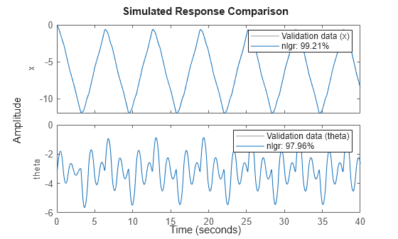
To evaluate the quality of the estimated model, simulate the estimated model and compare the measured and simulated output.

compare(z,nlgr); 

Generate State and Jacobian Function from Nonlinear Grey-Box Model

The multistage nonlinear MPC controller requires state and Jacobian functions defined as MATLAB® function files. You can use generateMATLABFunction to generate these function files from the estimated idnlgrey object. If you name the state function as stateFcnPend, then generateMATLABFunction names the corresponding Jacobian function as stateFcnPendJacobian.

generateMATLABFunction(nlgr,"stateFcnPend");

generateMATLABFunction creates the files stateFcnPend and stateFcnPendJacobian in your current folder to store the state function and its Jacobian, respectively. These functions use the estimated parameters and invoke the corresponding model ODE file (swingup_m.m).

Design Multistage Nonlinear MPC Using the Provided Functions

In this example, the plant has four states and one input. Set the prediction horizon h to 10 and sample time Ts to 0.1 s.

Create the multistage nonlinear MPC controller.

Ts = 0.1;
h = 10; 
msobj = nlmpcMultistage(h,4,1);
msobj.Ts = Ts; 

Specify the state and Jacobian functions obtained from generateMATLABFunction.

msobj.Model.StateFcn = "stateFcnPend";
msobj.Model.StateJacFcn = "stateFcnPendJacobian";
msobj.Model.IsContinuousTime = true; 

Specify the constraints on the cart position (first state) and the force (the manipulated variable).

msobj.ManipulatedVariables.Min = -100;
msobj.ManipulatedVariables.Max = 100;
msobj.States(1).Min = -10; 
msobj.States(1).Max = 10;
msobj.UseMVRate = true;

For this example, the cost function and the cost Jacobian functions for all stages are specified in the files myCostSwingup.m and myCostSwingupGradientFcn.m. In both functions, the last input argument p is the parameter vector containing the reference signal for the cart position and the pendulum angle.

type("myCostSwingup.m")

function cost =  myCostSwingup(stage,x,u,dmv,p)

Wmv = 0.01;
output = [x(1) x(3)]; 
ref = [p(1) p(2)];

if stage == 1
    cost = Wmv*(dmv^2);
elseif stage == 11
    cost = (output-ref)*(output-ref)';
else
    cost = (output-ref)*(output-ref)' + Wmv*(dmv^2);
end

end

type("myCostSwingupGradientFcn.m")

function [Gx, Gmv, Gdmv] = myCostSwingupGradientFcn(stage,x,u,dmv,p)

Wmv = 0.01; 
Gmv = zeros(1,1);
 
if stage == 1
    Gx = zeros(4,1);
    Gdmv = 2*Wmv*dmv;
elseif stage == 11
    Gx = [2*(x(1)-p(1)); 0; 2*(x(3)-p(2)); 0];
    Gdmv = zeros(1,1);
else
    Gx = [2*(x(1)-p(1)); 0; 2*(x(3)-p(2)); 0];
    Gdmv = 2*Wmv*dmv;
end

Set the cost function, the cost Jacobian function, and parameter length for each stage.

for ct=1:h+1
    msobj.Stages(ct).CostFcn = "myCostSwingup";
    msobj.Stages(ct).CostJacFcn = "myCostSwingupGradientFcn";
    msobj.Stages(ct).ParameterLength = 2;
end

Validate the state and cost function along with the cost Jacobian function.

simdata = getSimulationData(msobj);
simdata.StageParameter = repmat([0;-pi], h+1, 1); 
validateFcns(msobj,[0.1 0.2 -pi/2 0.3],0.4,simdata)

Model.StateFcn is OK.
Model.StateJacFcn is OK.
"CostFcn" of the following stages [1 2 3 4 5 6 7 8 9 10 11] are OK.
"CostJacFcn" of the following stages [1 2 3 4 5 6 7 8 9 10 11] are OK.
Analysis of user-provided model, cost, and constraint functions complete.

Validate Performance Using Closed-Loop Simulation in Simulink

Validate the performance of the controller by simulating it in a closed-loop with the original nonlinear model.

Open the Simulink® model of the closed-loop system.

mdl = "swingup_pendulum_multistageNMPC"; 
open_system(mdl)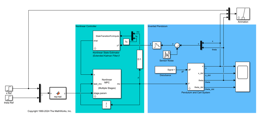

In this model, the Multistage MPC block is configured to use the msobj object in the workspace.

Run the simulation for 30 seconds.

open_system(mdl+'/Scope')
sim(mdl);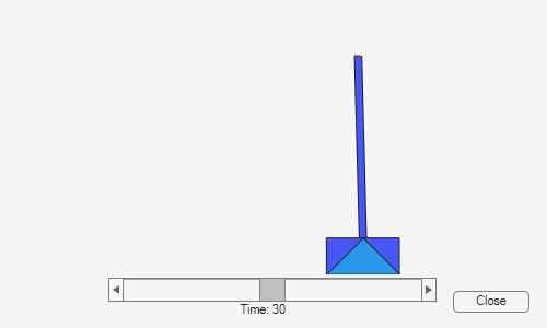

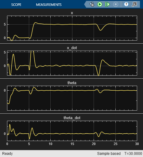
The simulation shows that the multistage nonlinear MPC controller designed from the estimated grey-box model can successfully swing-up and balance the pendulum in the inverted equilibrium, track the reference position, and reject disturbances.