Generate Sinusoidal Output from VCO
R2026bThis example shows how to obtain an ideal sine wave output at the frequency defined by a voltage-controlled oscillator (VCO). The example presents two approaches. In the discrete-time approach, you reuse the tuning characteristic of the Ring Oscillator VCO from Mixed-Signal Blockset™ -- the mapping from control voltage to instantaneous frequency -- and reconstruct a jitter-free sine wave from that frequency using phase accumulation. In the continuous-time approach, you build a standalone ideal sinusoidal VCO directly from the VCO equations. Both approaches focus on ideal behavior without modeling impairments like jitter or phase noise. Modeling noise is explicitly out of scope for this work.
Overview of Conversion Process for Discrete Time VCO
Start with the Mixed-Signal Blockset VCO block and configure it without enabling phase noise. Then use the command
set_param(gcb, 'LinkStatus', 'none')to make the block editable. The original Ring Oscillator VCO from Mixed-Signal Blockset™ outputs a pulse train whose frequency depends on the control voltage. Rather than using that pulse output, you tap the block's internal half-period signal (the same signal that sets the ring's oscillation rate) and use it to reconstruct a sine wave. The pulse-generating path is left intact but its output is not connected to the sine output. The reconstruction involves:Computing instantaneous frequency from the half-period.
Converting frequency to angular frequency.
Integrating angular frequency to obtain phase.
Wrapping phase between
 and
and  and adding an initial offset.
Generating sine wave from the accumulated phase.
Mathematical Foundations
The conversion relies on the following equations:
Instantaneous frequency:

Angular frequency:

Phase accumulation:

Phase wrapping:

Sine wave output:

Editing Ring Oscillator VCO
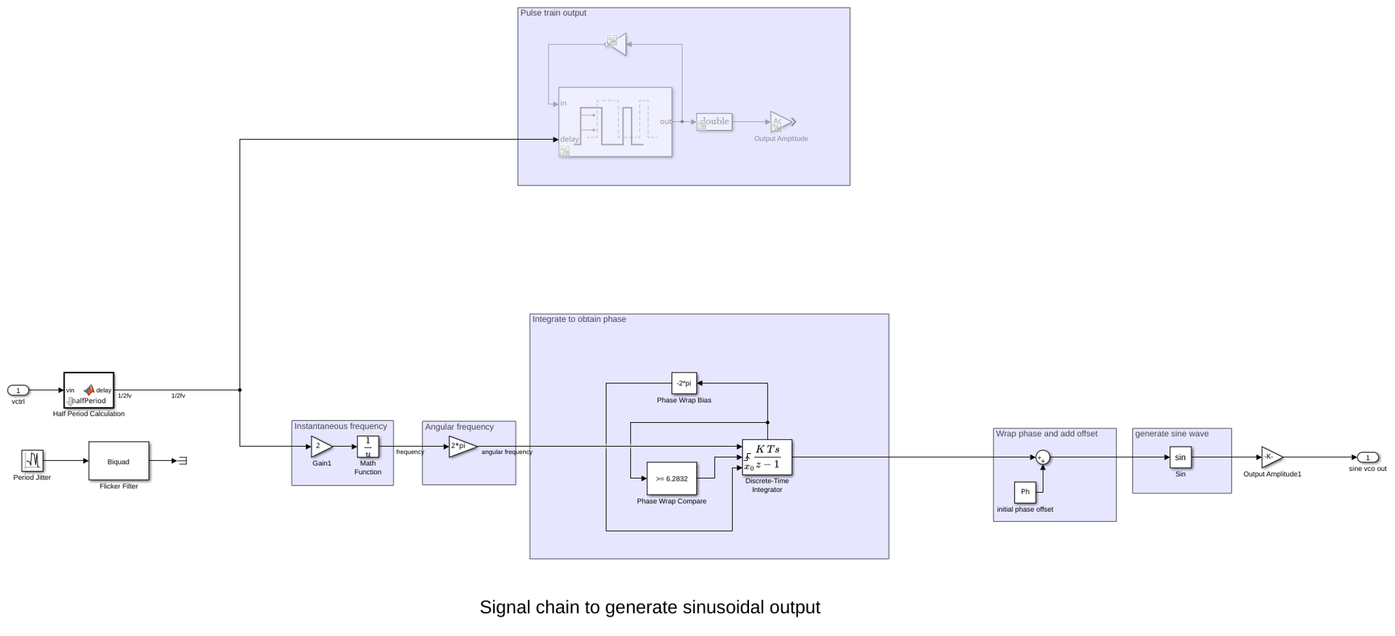
This section shows the inner structure of the Ring Oscillator VCO block. The block natively produces an ideal pulse train, and internally it computes the half-period of that pulse train from the control voltage. This half-period signal -- not the pulse train itself -- serves as the timing source you convert into a smooth sine wave.
Once you make the block editable by running the command set_param(gcb,'LinkStatus','none') , you can see the inner structure and locate the half-period signal produced by the Half Period Calculation subsystem.
You then reconstruct a sine wave from the half-period signal through the following steps:
1. Calculating Instantaneous Frequency
To monitor the time-varying performance of the VCO, the instantaneous frequency is calculated based on the half-period data  generated by the original ring oscillator VCO. Using half-period measurements allows for a higher-resolution frequency update rate compared to full-period measurements. The frequency is determined by doubling the half-period to approximate the full wavelength and taking the inverse which can be mathematically represented as
2. Deriving Angular Frequency
The next stage in the signal chain involves translating the instantaneous frequency into angular frequency via the formula This conversion bridges the domain gap between frequency and phase. While describes the number of cycles per second, phase processing requires the signal to be expressed in radians per second. By calculating  , you can establish the instantaneous rate of change of the phase, preparing the data for the integration process that follows.
3. Deriving Instantaneous Phase
The next step in the signal chain is the derivation of the instantaneous phase,  , by integrating the angular frequency over time: In the digital domain, this process is modeled as a continuous accumulation of phase increments. The Discrete-Time Integrator block is configured with the following specific parameters to ensure accurate conversion:
Integrator Method (Forward Euler): This method was selected for its computational efficiency and simplicity in handling discrete-time updates. It approximates the integral by adding the product of the current input and the sample time to the previous state.
Gain Value (1.0): A unity gain is applied to ensure the angular frequency is integrated directly without any additional scaling or attenuation.
Initial Condition (0): The integrator is initialized to zero to establish a consistent starting phase reference (
 ).
).Sample Time: For GHz-range VCOs, the sample time is set to an extremely small interval (e.g.,1/(128*2.5e9)). This significant oversampling is critical to capturing the fast-changing dynamics of the oscillator without aliasing artifacts.
Critical Implementation Considerations:
Sampling & Aliasing: For lower-frequency VCOs, the sample time can be relaxed, but it must strictly adhere to the Nyquist-Shannon sampling theorem to prevent signal distortion.
Numerical Stability: While Forward Euler is efficient, very small sample times can occasionally lead to numerical precision issues. If you observe any instability, you can either tune the solver settings or consider a more robust integration method like Trapezoidal.
Phase Wrapping (bounded accumulator): If left unbounded, the integrator state grows without limit and eventually overflows in a long-running simulation. A downstream modulo on the integrator output alone does not fix this -- it wraps the value feeding the sine, but the integrator's internal state keeps growing. Instead, the accumulated phase is wrapped inside the integrator itself, using a self-resetting feedback loop built from the following blocks (as shown in the signal chain figure):
Discrete-Time Integrator (with reset and external IC ports): The block is configured with an external reset port (Rising) and an external initial-condition port (
 ), enabled by turning on Show state port. These two extra input ports are what let the block reset its own accumulated state mid-simulation.
Phase Wrap Compare (Compare To Constant,
>= 6.2832): This block compares the integrator's state against (6.2832 rad). When the phase reaches or exceeds one full cycle, its output goes true and drives the integrator's reset port, triggering a reset on that step.Phase Wrap Bias (Bias,
-2*pi): This block subtracts from the current state and feeds the result to the integrator's port, so that on reset the phase continues from  rather than snapping back to zero. This preserves phase continuity across the wrap.
Why feed back from the state port, not the output port: Both the Compare and Bias feedback paths are taken from the integrator's state port (the small port that exposes the current state directly), not from its regular output port. Feeding the output port back into the reset/IC ports would create an algebraic loop, because the output would depend on the reset decision on the same time step. The state port breaks this dependency. Together, these blocks keep the accumulator bounded to
 indefinitely with no effect on the sine output, since the sine function is -periodic.
Dynamic Range: Because the state is wrapped by reset, output saturation limits are left at
 (no saturation). Wrapping via reset -- rather than clipping -- is what prevents variable overflow in long-duration simulations.
4. Wrapping Phase and Adding Offset
The accumulated phase is kept within a standard circle of [ , ] by wrapping the integrator state through its external reset port, as described above:  . An initial phase offset
  is then added to the wrapped phase to calibrate the wave's starting point. Wrapping the accumulator by reset (rather than applying a modulo only to the integrator output) ensures the state stays bounded and the signal phase resets correctly at the end of every cycle, preventing numerical overflow in long simulations.
5. Generating Sine Wave
The final stage of the signal chain transforms the instantaneous phase argument into a time-domain amplitude. By applying the trigonometric sine function to the wrapped phase input, you can compute the output using the equation: . This non-linear mapping converts the sawtooth-like phase ramp into a smooth, periodic sinusoidal waveform. The resulting signal oscillates within the range ![$[-A,+A]$](../../examples/msblks/GenerateSinusoidalOutputFromVCOExample_eq17395023407743059551.png) (where
(where  is the peak amplitude), making it spectrally pure and suitable for use as a local oscillator in RF mixers or communication systems.
Discrete Time VCO Simulation
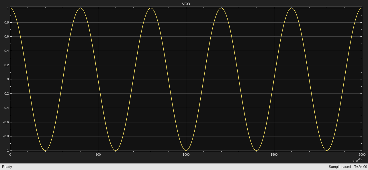
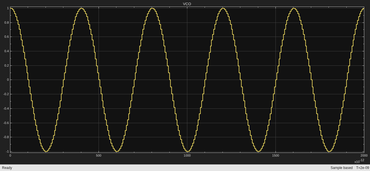
Run the attached model VCO_discrete which is configured with voltage sensitivity of 100MHz/Volt, free running frequency of 2.4GHz, amplitude of 1 Volt and with an initial phase of  /2 in the sinusoidal output. For a 1 Volt of control voltage we expect the VCO to be generating a sinusoidal output of 2.5GHz frequency. Accordingly, the sample time has been set as 1/(64*2.5e9) producing 64 points in one cycle of sine wave output
model='VCO_discrete';
load_system(model);
open_system([model,'/VCO']);
open_system([model,'/VCO/Variant Subsystem/DT-VCO/Ring Oscillator VCO'],'force','tab');
sim(model);
open_system([model,'/Scope']);
%
Overview of Conversion Process for Continuous Time VCO
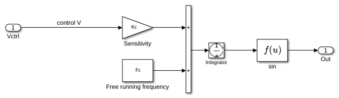
Unlike the discrete-time approach, the continuous-time VCO does not reuse the Ring Oscillator block. It is a standalone, ideal sinusoidal VCO built directly from the VCO equations below, sharing only the same mask parameters (free-running frequency, sensitivity, amplitude, and initial phase).
The instantaneous frequency for a voltage controlled oscillator is
![$f(t) = F_c + K_c V_{ctrl}(t) \quad [\mathrm{Hz}]$](../../examples/msblks/GenerateSinusoidalOutputFromVCOExample_eq06654448822292316953.png) where,
where,
 = free running frequency (Hz)
 = Voltage sensitivity of VCO (Hz/Volt)
 = Control voltage
Angular frequency and phase evolve as 
The sinusoidal output with amplitude and initial phase is:

In the implementation, the continuous-time Integrator integrates the instantaneous frequency  directly, so its state represents phase in cycles; the factor of (and the initial phase ) is applied afterward inside the sine function. To keep the accumulator bounded in long-running simulations, the Integrator block's built-in state wrapping is enabled with wrap limits of
  cycle. Because the continuous Integrator wraps its own state internally, no external reset logic or downstream modulo block is required. The mask interface (control voltage, free-running frequency , sensitivity , amplitude, and initial phase) is shared with the discrete-time VCO for convenience, but this continuous-time implementation is entirely independent of the Ring Oscillator block.
Above math is used to implement the VCO which is shown in the next section
Continuous Time VCO Simulation
model='VCO_continuous';
load_system(model);
open_system([model,'/VCO']);
open_system([model,'/VCO/Variant Subsystem/CT-VCO'],'force','tab');
sim(model);
open_system([model,'/Scope']);