Estimate Orientation Using GPS-Derived Yaw Measurements
This example shows how to define and use a custom sensor model for the insEKF object along with built-in sensor models. Using a custom yaw angle sensor, an accelerometer, and a gyroscope, this example uses the insEKF object to determine the orientation of a vehicle. You use the velocity from a GPS receiver to compute the yaw of the vehicle. Following a similar approach as shown in this example, you can develop custom sensor models for your own sensor fusion applications.
This example requires either the Sensor Fusion and Tracking Toolbox™ or the Navigation Toolbox™. This example also optionally uses MATLAB® Coder™ to accelerate filter tuning.
Problem Description
You are trying to estimate the orientation of a vehicle while it is moving. The only sensors available are an accelerometer, a gyroscope, and a GPS receiver that outputs a velocity estimate. You cannot use a magnetometer because there is a large amount of magnetic interference on the vehicle.
Approach
There are several tools available in the toolbox to determine orientation including
ecompassimufilterahrsfiltercomplementaryFilter
However, these filters require some combination of an accelerometer, a gyroscope, and/or a magnetometer. If you need to determine the absolute orientation (relative to True North) and do not have a magnetometer available, then none of these filters is ideal. The imufilter and complementaryFilter objects fuse accelerometer and gyroscope data, but they only provide a relative orientation. Furthermore, while these filters can estimate and compensate for the gyroscope bias, there is no additional sensor to help track the gyroscope bias for the yaw angle, which can yield a suboptimal estimate. Typically, a magnetometer is used to accomplish this. However, as mentioned, magnetometers cannot be used in situations with large, highly varying magnetic disturbances. (Note that the ahrsfilter object can handle mild magnetic disturbances over a short period of time).
In this example, to get the absolute orientation you use the GPS velocity estimate to determine the yaw angle. This yaw angle estimate can serve the same purpose as a magnetometer without the magnetic disturbance issues. You will build a custom sensor in the insEKF framework to model this GPS-based raw sensor.
Trajectory
First, you create a ground truth trajectory and simulate the sensor by using the exampleHelperMakeTrajectory and exampleHelperMakeIMUGPSData functions attached with this example:
groundTruth = exampleHelperMakeTrajectory;
originalSensorData = exampleHelperMakeIMUGPSData(groundTruth);
Retuned as a timetable, the original sensor data includes the accelerometer, gyroscope, and GPS velocity data. Transform the GPS velocity data into a yaw angle estimate.
velyaw = atan2(originalSensorData.GPSVelocity(:,2), originalSensorData.GPSVelocity(:,1));
The above results assume nonholonomic constraints. That is, they assume the vehicle is pointing in the direction of motion. This assumption is generally true some vehicles, such as a car, but not true for some other vehicles, such as a quadcopter.
Create Synthetic Yaw Angle Sensor Data
Yaw angle is difficult to work with because the yaw angle wraps at and . The angle jumping at the wrapping bound could cause divergence of the extended Kalman filter. To avoid this problem, convert the yaw angle to a quaternion.
velyaw(:,2) = 0; % set pitch and roll to 0
velyaw(:,3) = 0;
qyaw = quaternion(velyaw, 'euler', 'ZYX', 'frame');
A common convention is to force the quaternion to have a positive real part
isNegQuat = parts(qyaw) < 0; % Find quaternions with a non-negative real part
qyaw(isNegQuat) = -qyaw(isNegQuat); % Invert the negative quaternions.
Note that when the insEKF object tracks a 4-element Orientation state as in this example, it assumes the Orientation state is a quaternion and enforces the quaternion to be normalized and have a positive real part. You can disable this rule by calling the state something else, like "Attitude".
Now you can build the timetable of the sensor data to be fused.
sensorData = removevars(originalSensorData, 'GPSVelocity');
sensorData = addvars(sensorData,compact(qyaw),'NewVariableNames','YawSensor');
Create an insEKF Sensor for Fusing Yaw Angle
To fuse the yaw angle quaternion, you customize a sensor model and use it along with the insAccelerometer and insGyroscope objects in the insEKF object. To customize the sensor model, you create a class that inherits from the positioning.INSSensorModel interface class and implement the measurement method. Name the class exampleHelperYawSensor
classdef exampleHelperYawSensor < positioning.INSSensorModel
%EXAMPLEHELPERYAWSENSOR Yaw angle as quaternion sensor
% This class is for internal use only. It may be removed in the future.


%   Copyright 2021 The MathWorks, Inc.

    methods
        function z = measurement(~, filt)
            % Return an estimate of the measurement based on the
            % state vector of the filter saved in filt.State.
            %
            % The measurement is just the quaternion converted from the yaw
            % of the orientation estimate, assuming roll=0 and pitch=0.

            q = quaternion(stateparts(filt, "Orientation"));
            eul  = euler(q, 'ZYX', 'frame');
            yawquat = quaternion([eul(1) 0 0], 'euler', 'ZYX', 'frame');

            % Enforce a positive quaternion convention
            if parts(yawquat) < 0
                yawquat = -yawquat;
            end

            % Return a compacted quaternion
            z = compact(yawquat);
        end
    end
end
Now use a exampleHelperYawSensor object alongside an insAccelerometer object and an insGyroscope object to construct the insEKF object.
opts = insOptions(SensorNamesSource='property', SensorNames={'Accelerometer', 'Gyroscope', 'YawSensor'});
filt = insEKF(insAccelerometer, insGyroscope, exampleHelperYawSensor, insMotionOrientation, opts);
Initialize the filter using the stateparts and statecovparts object functions.
stateparts(filt, 'Orientation', sensorData.YawSensor(1,:));
statecovparts(filt,'Accelerometer_Bias', 1e-3);
statecovparts(filt,'Gyroscope_Bias', 1e-3);
Filter Tuning
You can use the tune object function to find the optimal noise parameters for the insEKF object. You can directly call the tune object function, or you can use a MEX-accelerated cost function with MATLAB Coder.
% Trim ground truth to just contain the Orientation for tuning.
trimmedGroundTruth = timetable(groundTruth.Orientation, ...
    SampleRate=groundTruth.Properties.SampleRate, ...
    VariableNames={'Orientation'});

% Use MATLAB Coder to accelerate tuning by MEXing the cost function.
% To run the MATLAB Coder accelerated path, prior to running the example,
% type:
%   exampleHelperUseAcceleratedTuning(true);
% To avoid using MATLAB Coder, prior to the example, type:
%   exampleHelperUseAcceleratedTuning(false);
% By default, the example will not tune the filter live and will not use
% MATLAB Coder.

% Select the accelerated tuning option.
acceleratedTuning = exampleHelperUseAcceleratedTuning();

if acceleratedTuning
    createTunerCostTemplate(filt); % A new cost function in the editor
    % Save and close the file
    doc = matlab.desktop.editor.getActive;
    doc.saveAs(fullfile(pwd, 'tunercost.m'));
    doc.close;
    % Find the first parameter for codegen
    p = tunerCostFcnParam(filt); %#ok<NASGU>
    % Now generate a mex file
    codegen tunercost.m -args {p, sensorData, trimmedGroundTruth};
    % Use the Custom Cost Function and run the tuner for 20 iterations
    tunerIters = 20;
    cfg = tunerconfig(filt, MaxIterations=tunerIters, ...
        Cost='custom', CustomCostFcn=@tunercost_mex, ...
        StepForward=1.5, ...
        ObjectiveLimit=0.0001, ...
        FunctionTolerance=1e-6, ...
        Display='none');

    mnoise = tunernoise(filt);
    tunedmn = tune(filt, mnoise, sensorData, trimmedGroundTruth, cfg);
else
    % Use optimal parameters obtained separately.
    tunedmn = struct(...
        'AccelerometerNoise', 0.7786515625000000, ...
        'GyroscopeNoise', 167.8674323338237, ...
        'YawSensorNoise', 1.003122320344434);

    adp = diag([...
          1.265000000000000;
          1.181989791398048;
          0.735171900658607;
          0.765000000000000;
          0.026248409763699;
          0.154586330266264;
          31.823154516336434;
          0.000546245218270;
          5.517012554348883;
          0.809085937500000;
          0.139035477206961;
          41.340145917279159;
          0.592875000000000]);
    filt.AdditiveProcessNoise = adp;
end
Fuse Data and Compare to Ground Truth
Batch fuse the data with the estimateStates object function.
est = estimateStates(filt, sensorData, tunedmn)
est=13500×5 timetable
      Time       Orientation                 AngularVelocity                           Accelerometer_Bias                            Gyroscope_Bias                StateCovariance
    ________    ______________    ______________________________________    _________________________________________    ______________________________________    _______________

    0 sec       1×1 quaternion    0.00029964     0.0003257    0.00033221     3.1017e-08    -2.3517e-24    -1.2416e-09    2.9964e-07     3.257e-07    3.3221e-07    {13×13 double}
    0.01 sec    1×1 quaternion    0.00058811     0.0010514    0.00077335    -1.7319e-10    -1.9136e-05     1.5274e-06    1.0727e-06    0.00013317    2.6591e-06    {13×13 double}
    0.02 sec    1×1 quaternion     0.0010153     0.0011293     0.0012812     1.1835e-08     5.0402e-05     4.4661e-06    2.2303e-06     0.0003694    6.6701e-06    {13×13 double}
    0.03 sec    1×1 quaternion     0.0013953     0.0014522     0.0019019     1.0275e-08     9.5573e-05     2.0662e-06    3.7974e-06    0.00073969    1.2675e-05    {13×13 double}
    0.04 sec    1×1 quaternion     0.0017109     0.0015025     0.0025803     2.3834e-08     0.00010594     6.3287e-06    5.7708e-06     0.0012283    2.0107e-05    {13×13 double}
    0.05 sec    1×1 quaternion       0.00205     0.0019622     0.0033511     1.4978e-08     0.00012105     5.2769e-06    8.2924e-06     0.0018652    2.9309e-05    {13×13 double}
    0.06 sec    1×1 quaternion     0.0020261     0.0023534     0.0041042     8.8652e-09    -6.6667e-05     1.5446e-06    1.1182e-05     0.0025908    3.8877e-05    {13×13 double}
    0.07 sec    1×1 quaternion     0.0026568     0.0026599     0.0050163     8.3994e-09     0.00012693      4.528e-06    1.4392e-05     0.0034661    5.0998e-05    {13×13 double}
    0.08 sec    1×1 quaternion     0.0027766     0.0029837     0.0058779      2.101e-09     3.3626e-05     1.1473e-05    1.7889e-05     0.0042033    6.2921e-05    {13×13 double}
    0.09 sec    1×1 quaternion     0.0032068     0.0030261     0.0068784     1.3912e-08     0.00011826     1.7097e-05    2.1816e-05     0.0051831    7.7173e-05    {13×13 double}
    0.1 sec     1×1 quaternion     0.0031981     0.0032051      0.007876      1.643e-08    -7.5163e-05     1.2083e-05    2.6806e-05     0.0061659    9.1711e-05    {13×13 double}
    0.11 sec    1×1 quaternion     0.0036603     0.0032823      0.008879     2.4021e-08     3.2796e-05     1.2375e-05    3.1437e-05       0.00716    0.00010671    {13×13 double}
    0.12 sec    1×1 quaternion      0.003734     0.0034359     0.0099138     2.7443e-08    -9.4583e-05     8.6765e-06    3.6787e-05     0.0083283     0.0001224    {13×13 double}
    0.13 sec    1×1 quaternion     0.0039583     0.0036587      0.011055     2.6296e-08    -0.00012251     3.6091e-06    4.2167e-05     0.0095194    0.00014002    {13×13 double}
    0.14 sec    1×1 quaternion     0.0040944     0.0040022      0.012244     1.7306e-08     -0.0002173      2.531e-06    4.8518e-05       0.01074    0.00015864    {13×13 double}
    0.15 sec    1×1 quaternion     0.0044477     0.0040462      0.013476     2.4033e-08    -0.00015984     8.1767e-06    5.4321e-05      0.011837    0.00017817    {13×13 double}
      ⋮
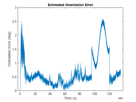
Compare the estimated orientation to ground truth orientation. Plot the quaternion distance between the estimated and true orientations.
% Convert compacted quaternions to regular quaternions
estOrient = quaternion(est.Orientation);

d = rad2deg(dist(estOrient, groundTruth.Orientation));
plot(groundTruth.Time, d);
xlabel('Time (s)')
ylabel('Orientation Error (deg)');
title('Estimated Orientation Error');
snapnow;
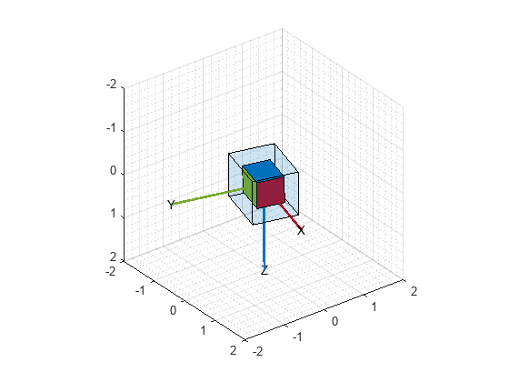
From the results, the estimated orientation error is low overall. There is a small bump in the error around 100 seconds, which is likely due to a slight inflection in the ground truth yaw angle at the time. But overall, this is a good orientation estimate result for many applications. You can visualize the estimated orientation using the poseplot function.
p = poseplot(estOrient(1));
for ii=2:numel(estOrient)
    p.Orientation = estOrient(ii);
    drawnow limitrate;
end
Conclusion
In this example, you learned how to customize a sensor and add it to the insEKF framework. Custom sensors can integrate with the built-in sensors like insAccelerometer and insGyroscope. You also learned how to use the tune object function to find optimal noise parameters and improve the filtering results.