Main Content

alexnet

AlexNet convolutional neural network

  • AlexNet network architecture

Description

AlexNet is a convolutional neural network that is 8 layers deep. You can load a pretrained version of the network trained on more than a million images from the ImageNet database [1]. The pretrained network can classify images into 1000 object categories, such as keyboard, mouse, pencil, and many animals. As a result, the network has learned rich feature representations for a wide range of images. The network has an image input size of 227-by-227. For more pretrained networks in MATLAB®, see Pretrained Deep Neural Networks.

You can use classify to classify new images using the AlexNet network. Follow the steps of Classify Image Using GoogLeNet and replace GoogLeNet with AlexNet.

For a free hands-on introduction to practical deep learning methods, see Deep Learning Onramp.

example

net = alexnet returns an AlexNet network trained on the ImageNet data set.

This function requires Deep Learning Toolbox™ Model for AlexNet Network support package. If this support package is not installed, the function provides a download link. Alternatively, see Deep Learning Toolbox Model for AlexNet Network.

For more pretrained networks in MATLAB, see Pretrained Deep Neural Networks.

net = alexnet('Weights','imagenet') returns an AlexNet network trained on the ImageNet data set. This syntax is equivalent to net = alexnet.

layers = alexnet('Weights','none') returns the untrained AlexNet network architecture. The untrained model does not require the support package.

Examples

collapse all

Download and install Deep Learning Toolbox Model for AlexNet Network support package.

Type alexnet at the command line.

alexnet

If Deep Learning Toolbox Model for AlexNet Network support package is not installed, then the function provides a link to the required support package in the Add-On Explorer. To install the support package, click the link, and then click Install. Check that the installation is successful by typing alexnet at the command line.

alexnet
ans = 

  SeriesNetwork with properties:

    Layers: [25×1 nnet.cnn.layer.Layer]

If the required support package is installed, then the function returns a SeriesNetwork object.

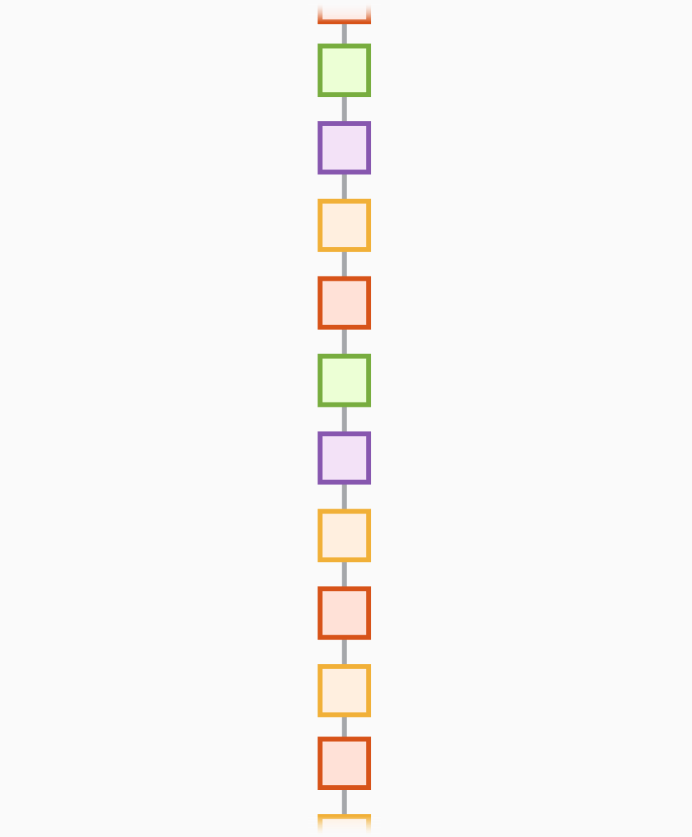
Visualize the network using Deep Network Designer.

deepNetworkDesigner(alexnet)

Explore other pretrained neural networks in Deep Network Designer by clicking New.

Deep Network Designer start page showing available pretrained neural networks

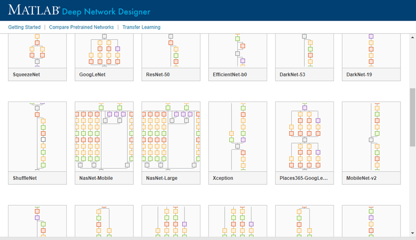
If you need to download a neural network, pause on the desired neural network and click Install to open the Add-On Explorer.

This example shows how to fine-tune a pretrained AlexNet convolutional neural network to perform classification on a new collection of images.

AlexNet has been trained on over a million images and can classify images into 1000 object categories (such as keyboard, coffee mug, pencil, and many animals). The network has learned rich feature representations for a wide range of images. The network takes an image as input and outputs a label for the object in the image together with the probabilities for each of the object categories.

Transfer learning is commonly used in deep learning applications. You can take a pretrained network and use it as a starting point to learn a new task. Fine-tuning a network with transfer learning is usually much faster and easier than training a network with randomly initialized weights from scratch. You can quickly transfer learned features to a new task using a smaller number of training images.

Load Data

Unzip and load the new images as an image datastore. imageDatastore automatically labels the images based on folder names and stores the data as an ImageDatastore object. An image datastore enables you to store large image data, including data that does not fit in memory, and efficiently read batches of images during training of a convolutional neural network.

unzip('MerchData.zip');
imds = imageDatastore('MerchData', ...
    'IncludeSubfolders',true, ...
    'LabelSource','foldernames');

Divide the data into training and validation data sets. Use 70% of the images for training and 30% for validation. splitEachLabel splits the images datastore into two new datastores.

[imdsTrain,imdsValidation] = splitEachLabel(imds,0.7,'randomized');

This very small data set now contains 55 training images and 20 validation images. Display some sample images.

numTrainImages = numel(imdsTrain.Labels);
idx = randperm(numTrainImages,16);
figure
for i = 1:16
    subplot(4,4,i)
    I = readimage(imdsTrain,idx(i));
    imshow(I)
end

Load Pretrained Network

Load the pretrained AlexNet neural network. If Deep Learning Toolbox™ Model for AlexNet Network is not installed, then the software provides a download link. AlexNet is trained on more than one million images and can classify images into 1000 object categories, such as keyboard, mouse, pencil, and many animals. As a result, the model has learned rich feature representations for a wide range of images.

net = alexnet;

Use analyzeNetwork to display an interactive visualization of the network architecture and detailed information about the network layers.

analyzeNetwork(net)

The first layer, the image input layer, requires input images of size 227-by-227-by-3, where 3 is the number of color channels.

inputSize = net.Layers(1).InputSize
inputSize = 1×3

   227   227     3

Replace Final Layers

The last three layers of the pretrained network net are configured for 1000 classes. These three layers must be fine-tuned for the new classification problem. Extract all layers, except the last three, from the pretrained network.

layersTransfer = net.Layers(1:end-3);

Transfer the layers to the new classification task by replacing the last three layers with a fully connected layer, a softmax layer, and a classification output layer. Specify the options of the new fully connected layer according to the new data. Set the fully connected layer to have the same size as the number of classes in the new data. To learn faster in the new layers than in the transferred layers, increase the WeightLearnRateFactor and BiasLearnRateFactor values of the fully connected layer.

numClasses = numel(categories(imdsTrain.Labels))
numClasses = 5
layers = [
    layersTransfer
    fullyConnectedLayer(numClasses,'WeightLearnRateFactor',20,'BiasLearnRateFactor',20)
    softmaxLayer
    classificationLayer];

Train Network

The network requires input images of size 227-by-227-by-3, but the images in the image datastores have different sizes. Use an augmented image datastore to automatically resize the training images. Specify additional augmentation operations to perform on the training images: randomly flip the training images along the vertical axis, and randomly translate them up to 30 pixels horizontally and vertically. Data augmentation helps prevent the network from overfitting and memorizing the exact details of the training images.

pixelRange = [-30 30];
imageAugmenter = imageDataAugmenter( ...
    'RandXReflection',true, ...
    'RandXTranslation',pixelRange, ...
    'RandYTranslation',pixelRange);
augimdsTrain = augmentedImageDatastore(inputSize(1:2),imdsTrain, ...
    'DataAugmentation',imageAugmenter);

To automatically resize the validation images without performing further data augmentation, use an augmented image datastore without specifying any additional preprocessing operations.

augimdsValidation = augmentedImageDatastore(inputSize(1:2),imdsValidation);

Specify the training options. For transfer learning, keep the features from the early layers of the pretrained network (the transferred layer weights). To slow down learning in the transferred layers, set the initial learning rate to a small value. In the previous step, you increased the learning rate factors for the fully connected layer to speed up learning in the new final layers. This combination of learning rate settings results in fast learning only in the new layers and slower learning in the other layers. When performing transfer learning, you do not need to train for as many epochs. An epoch is a full training cycle on the entire training data set. Specify the mini-batch size and validation data. The software validates the network every ValidationFrequency iterations during training.

options = trainingOptions('sgdm', ...
    'MiniBatchSize',10, ...
    'MaxEpochs',6, ...
    'InitialLearnRate',1e-4, ...
    'Shuffle','every-epoch', ...
    'ValidationData',augimdsValidation, ...
    'ValidationFrequency',3, ...
    'Verbose',false, ...
    'Plots','training-progress');

Train the network that consists of the transferred and new layers. By default, trainNetwork uses a GPU if one is available, otherwise, it uses a CPU. Training on a GPU requires Parallel Computing Toolbox™ and a supported GPU device. For information on supported devices, see GPU Computing Requirements (Parallel Computing Toolbox). You can also specify the execution environment by using the 'ExecutionEnvironment' name-value pair argument of trainingOptions.

netTransfer = trainNetwork(augimdsTrain,layers,options);

Classify Validation Images

Classify the validation images using the fine-tuned network.

[YPred,scores] = classify(netTransfer,augimdsValidation);

Display four sample validation images with their predicted labels.

idx = randperm(numel(imdsValidation.Files),4);
figure
for i = 1:4
    subplot(2,2,i)
    I = readimage(imdsValidation,idx(i));
    imshow(I)
    label = YPred(idx(i));
    title(string(label));
end

Calculate the classification accuracy on the validation set. Accuracy is the fraction of labels that the network predicts correctly.

YValidation = imdsValidation.Labels;
accuracy = mean(YPred == YValidation)
accuracy = 1

For tips on improving classification accuracy, see Deep Learning Tips and Tricks.

Read, resize, and classify an image using AlexNet. First, load a pretrained AlexNet model.

net = alexnet;

Read the image using imread.

I = imread('peppers.png');
figure
imshow(I)

The pretrained model requires the image size to be the same as the input size of the network. Determine the input size of the network using the InputSize property of the first layer of the network.

sz = net.Layers(1).InputSize
sz = 1×3

   227   227     3

Resize the image to the input size of the network.

I = imresize(I,sz(1:2));
figure
imshow(I)

Classify the image using classify.

label = classify(net,I)
label = categorical
     bell pepper 

Show the image and classification result together.

figure
imshow(I)
title(label)

This example shows how to extract learned image features from a pretrained convolutional neural network, and use those features to train an image classifier. Feature extraction is the easiest and fastest way to use the representational power of pretrained deep networks. For example, you can train a support vector machine (SVM) using fitcecoc (Statistics and Machine Learning Toolbox™) on the extracted features. Because feature extraction only requires a single pass through the data, it is a good starting point if you do not have a GPU to accelerate network training with.

Load Data

Unzip and load the sample images as an image datastore. imageDatastore automatically labels the images based on folder names and stores the data as an ImageDatastore object. An image datastore lets you store large image data, including data that does not fit in memory. Split the data into 70% training and 30% test data.

unzip('MerchData.zip');

imds = imageDatastore('MerchData', ...
    'IncludeSubfolders',true, ...
    'LabelSource','foldernames');

[imdsTrain,imdsTest] = splitEachLabel(imds,0.7,'randomized');

There are now 55 training images and 20 validation images in this very small data set. Display some sample images.

numImagesTrain = numel(imdsTrain.Labels);
idx = randperm(numImagesTrain,16);

for i = 1:16
    I{i} = readimage(imdsTrain,idx(i));
end

figure
imshow(imtile(I))

Load Pretrained Network

Load a pretrained AlexNet network. If the Deep Learning Toolbox Model for AlexNet Network support package is not installed, then the software provides a download link. AlexNet is trained on more than a million images and can classify images into 1000 object categories. For example, keyboard, mouse, pencil, and many animals. As a result, the model has learned rich feature representations for a wide range of images.

net = alexnet;

Display the network architecture. The network has five convolutional layers and three fully connected layers.

net.Layers
ans = 
  25x1 Layer array with layers:

     1   'data'     Image Input                   227x227x3 images with 'zerocenter' normalization
     2   'conv1'    Convolution                   96 11x11x3 convolutions with stride [4  4] and padding [0  0  0  0]
     3   'relu1'    ReLU                          ReLU
     4   'norm1'    Cross Channel Normalization   cross channel normalization with 5 channels per element
     5   'pool1'    Max Pooling                   3x3 max pooling with stride [2  2] and padding [0  0  0  0]
     6   'conv2'    Grouped Convolution           2 groups of 128 5x5x48 convolutions with stride [1  1] and padding [2  2  2  2]
     7   'relu2'    ReLU                          ReLU
     8   'norm2'    Cross Channel Normalization   cross channel normalization with 5 channels per element
     9   'pool2'    Max Pooling                   3x3 max pooling with stride [2  2] and padding [0  0  0  0]
    10   'conv3'    Convolution                   384 3x3x256 convolutions with stride [1  1] and padding [1  1  1  1]
    11   'relu3'    ReLU                          ReLU
    12   'conv4'    Grouped Convolution           2 groups of 192 3x3x192 convolutions with stride [1  1] and padding [1  1  1  1]
    13   'relu4'    ReLU                          ReLU
    14   'conv5'    Grouped Convolution           2 groups of 128 3x3x192 convolutions with stride [1  1] and padding [1  1  1  1]
    15   'relu5'    ReLU                          ReLU
    16   'pool5'    Max Pooling                   3x3 max pooling with stride [2  2] and padding [0  0  0  0]
    17   'fc6'      Fully Connected               4096 fully connected layer
    18   'relu6'    ReLU                          ReLU
    19   'drop6'    Dropout                       50% dropout
    20   'fc7'      Fully Connected               4096 fully connected layer
    21   'relu7'    ReLU                          ReLU
    22   'drop7'    Dropout                       50% dropout
    23   'fc8'      Fully Connected               1000 fully connected layer
    24   'prob'     Softmax                       softmax
    25   'output'   Classification Output         crossentropyex with 'tench' and 999 other classes

The first layer, the image input layer, requires input images of size 227-by-227-by-3, where 3 is the number of color channels.

inputSize = net.Layers(1).InputSize
inputSize = 1×3

   227   227     3

Extract Image Features

The network constructs a hierarchical representation of input images. Deeper layers contain higher-level features, constructed using the lower-level features of earlier layers. To get the feature representations of the training and test images, use activations on the fully connected layer 'fc7'. To get a lower-level representation of the images, use an earlier layer in the network.

The network requires input images of size 227-by-227-by-3, but the images in the image datastores have different sizes. To automatically resize the training and test images before they are input to the network, create augmented image datastores, specify the desired image size, and use these datastores as input arguments to activations.

augimdsTrain = augmentedImageDatastore(inputSize(1:2),imdsTrain);
augimdsTest = augmentedImageDatastore(inputSize(1:2),imdsTest);

layer = 'fc7';
featuresTrain = activations(net,augimdsTrain,layer,'OutputAs','rows');
featuresTest = activations(net,augimdsTest,layer,'OutputAs','rows');

Extract the class labels from the training and test data.

YTrain = imdsTrain.Labels;
YTest = imdsTest.Labels;

Fit Image Classifier

Use the features extracted from the training images as predictor variables and fit a multiclass support vector machine (SVM) using fitcecoc (Statistics and Machine Learning Toolbox).

mdl = fitcecoc(featuresTrain,YTrain);

Classify Test Images

Classify the test images using the trained SVM model and the features extracted from the test images.

YPred = predict(mdl,featuresTest);

Display four sample test images with their predicted labels.

idx = [1 5 10 15];
figure
for i = 1:numel(idx)
    subplot(2,2,i)
    I = readimage(imdsTest,idx(i));
    label = YPred(idx(i));
    
    imshow(I)
    title(label)
end

Calculate the classification accuracy on the test set. Accuracy is the fraction of labels that the network predicts correctly.

accuracy = mean(YPred == YTest)
accuracy = 1

This SVM has high accuracy. If the accuracy is not high enough using feature extraction, then try transfer learning instead.

Output Arguments

collapse all

Pretrained AlexNet convolutional neural network, returned as a SeriesNetwork object.

Untrained AlexNet convolutional neural network architecture, returned as a Layer array.

Tips

References

[1] ImageNet. http://www.image-net.org

[2] Russakovsky, O., Deng, J., Su, H., et al. "ImageNet Large Scale Visual Recognition Challenge." International Journal of Computer Vision (IJCV). Vol 115, Issue 3, 2015, pp. 211–252

[3] Krizhevsky, Alex, Ilya Sutskever, and Geoffrey E. Hinton. "ImageNet Classification with Deep Convolutional Neural Networks." Communications of the ACM 60, no. 6 (May 24, 2017): 84–90. https://doi.org/10.1145/3065386

[4] BVLC AlexNet Model. https://github.com/BVLC/caffe/tree/master/models/bvlc_alexnet

Extended Capabilities

Version History

Introduced in R2017a