Main Content

trainAutoencoder

Train an autoencoder

Description

example

autoenc = trainAutoencoder(X) returns an autoencoder, autoenc, trained using the training data in X.

autoenc = trainAutoencoder(X,hiddenSize) returns an autoencoder autoenc, with the hidden representation size of hiddenSize.

example

autoenc = trainAutoencoder(___,Name,Value) returns an autoencoder autoenc, for any of the above input arguments with additional options specified by one or more Name,Value pair arguments.

For example, you can specify the sparsity proportion or the maximum number of training iterations.

Examples

collapse all

Load the sample data.

X = abalone_dataset;

X is an 8-by-4177 matrix defining eight attributes for 4177 different abalone shells: sex (M, F, and I (for infant)), length, diameter, height, whole weight, shucked weight, viscera weight, shell weight. For more information on the dataset, type help abalone_dataset in the command line.

Train a sparse autoencoder with default settings.

autoenc = trainAutoencoder(X);

Figure Neural Network Training (19-Aug-2023 11:46:34) contains an object of type uigridlayout.

Reconstruct the abalone shell ring data using the trained autoencoder.

XReconstructed = predict(autoenc,X);

Compute the mean squared reconstruction error.

mseError = mse(X-XReconstructed)
mseError = 0.0167

Load the sample data.

X = abalone_dataset;

X is an 8-by-4177 matrix defining eight attributes for 4177 different abalone shells: sex (M, F, and I (for infant)), length, diameter, height, whole weight, shucked weight, viscera weight, shell weight. For more information on the dataset, type help abalone_dataset in the command line.

Train a sparse autoencoder with hidden size 4, 400 maximum epochs, and linear transfer function for the decoder.

autoenc = trainAutoencoder(X,4,'MaxEpochs',400,...
'DecoderTransferFunction','purelin');

Figure Neural Network Training (19-Aug-2023 11:40:52) contains an object of type uigridlayout.

Reconstruct the abalone shell ring data using the trained autoencoder.

XReconstructed = predict(autoenc,X);

Compute the mean squared reconstruction error.

mseError = mse(X-XReconstructed)
mseError = 0.0044

Generate the training data.

rng(0,'twister'); % For reproducibility
n = 1000;
r = linspace(-10,10,n)';
x = 1 + r*5e-2 + sin(r)./r + 0.2*randn(n,1);

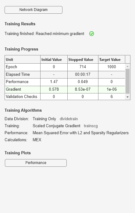
Train autoencoder using the training data.

hiddenSize = 25;
autoenc = trainAutoencoder(x',hiddenSize,...
        'EncoderTransferFunction','satlin',...
        'DecoderTransferFunction','purelin',...
        'L2WeightRegularization',0.01,...
        'SparsityRegularization',4,...
        'SparsityProportion',0.10);

Figure Neural Network Training (19-Aug-2023 11:42:57) contains an object of type uigridlayout.

Generate the test data.

n = 1000;
r = sort(-10 + 20*rand(n,1));
xtest = 1 + r*5e-2 + sin(r)./r + 0.4*randn(n,1);

Predict the test data using the trained autoencoder, autoenc.

xReconstructed = predict(autoenc,xtest');

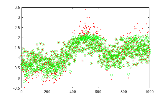
Plot the actual test data and the predictions.

figure;
plot(xtest,'r.');
hold on
plot(xReconstructed,'go');

Figure contains an axes object. The axes object contains 2 objects of type line. One or more of the lines displays its values using only markers

Load the training data.

XTrain = digitTrainCellArrayData;

The training data is a 1-by-5000 cell array, where each cell containing a 28-by-28 matrix representing a synthetic image of a handwritten digit.

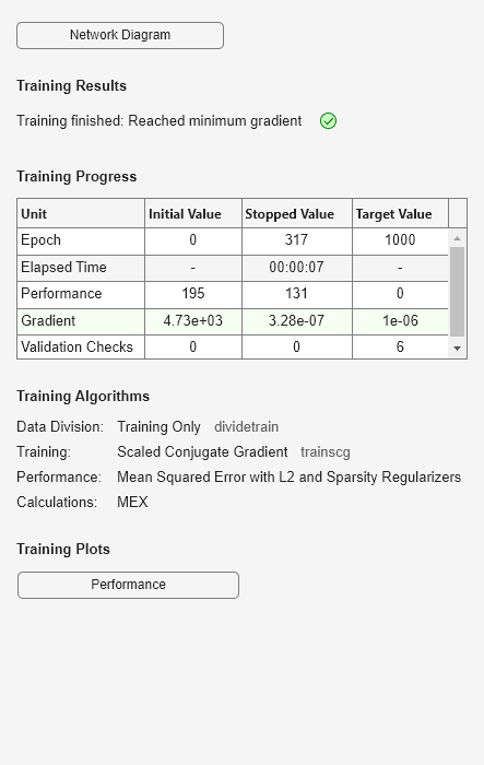
Train an autoencoder with a hidden layer containing 25 neurons.

hiddenSize = 25;
autoenc = trainAutoencoder(XTrain,hiddenSize,...
        'L2WeightRegularization',0.004,...
        'SparsityRegularization',4,...
        'SparsityProportion',0.15);

Load the test data.

XTest = digitTestCellArrayData;

The test data is a 1-by-5000 cell array, with each cell containing a 28-by-28 matrix representing a synthetic image of a handwritten digit.

Reconstruct the test image data using the trained autoencoder, autoenc.

xReconstructed = predict(autoenc,XTest);

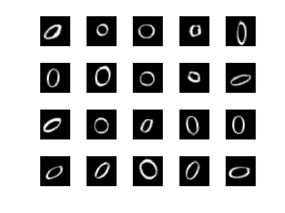
View the actual test data.

figure;
for i = 1:20
    subplot(4,5,i);
    imshow(XTest{i});
end

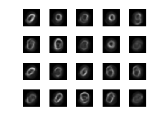
View the reconstructed test data.

figure;
for i = 1:20
    subplot(4,5,i);
    imshow(xReconstructed{i});
end

Input Arguments

collapse all

Training data, specified as a matrix of training samples or a cell array of image data. If X is a matrix, then each column contains a single sample. If X is a cell array of image data, then the data in each cell must have the same number of dimensions. The image data can be pixel intensity data for gray images, in which case, each cell contains an m-by-n matrix. Alternatively, the image data can be RGB data, in which case, each cell contains an m-by-n-3 matrix.

Data Types: single | double | cell

Size of hidden representation of the autoencoder, specified as a positive integer value. This number is the number of neurons in the hidden layer.

Data Types: single | double

Name-Value Arguments

Specify optional pairs of arguments as Name1=Value1,...,NameN=ValueN, where Name is the argument name and Value is the corresponding value. Name-value arguments must appear after other arguments, but the order of the pairs does not matter.

Before R2021a, use commas to separate each name and value, and enclose Name in quotes.

Example: 'EncoderTransferFunction','satlin','L2WeightRegularization',0.05 specifies the transfer function for the encoder as the positive saturating linear transfer function and the L2 weight regularization as 0.05.

Transfer function for the encoder, specified as the comma-separated pair consisting of 'EncoderTransferFunction' and one of the following.

Transfer Function OptionDefinition
'logsig'

Logistic sigmoid function

f(z)=11+ez

'satlin'

Positive saturating linear transfer function

f(z)={0,if z0z,if 0<z<11,if z1

Example: 'EncoderTransferFunction','satlin'

Transfer function for the decoder, specified as the comma-separated pair consisting of 'DecoderTransferFunction' and one of the following.

Transfer Function OptionDefinition
'logsig'

Logistic sigmoid function

f(z)=11+ez

'satlin'

Positive saturating linear transfer function

f(z)={0,if z0z,if 0<z<11,if z1

'purelin'

Linear transfer function

f(z)=z

Example: 'DecoderTransferFunction','purelin'

Maximum number of training epochs or iterations, specified as the comma-separated pair consisting of 'MaxEpochs' and a positive integer value.

Example: 'MaxEpochs',1200

The coefficient for the L2 weight regularizer in the cost function (LossFunction), specified as the comma-separated pair consisting of 'L2WeightRegularization' and a positive scalar value.

Example: 'L2WeightRegularization',0.05

Loss function to use for training, specified as the comma-separated pair consisting of 'LossFunction' and 'msesparse'. It corresponds to the mean squared error function adjusted for training a sparse autoencoder as follows:

E=1Nn=1Nk=1K(xknx^kn)2mean squared error+λ*ΩweightsL2regularization+β*Ωsparsitysparsityregularization,

where λ is the coefficient for the L2 regularization term and β is the coefficient for the sparsity regularization term. You can specify the values of λ and β by using the L2WeightRegularization and SparsityRegularization name-value pair arguments, respectively, while training an autoencoder.

Indicator to show the training window, specified as the comma-separated pair consisting of 'ShowProgressWindow' and either true or false.

Example: 'ShowProgressWindow',false

Desired proportion of training examples a neuron reacts to, specified as the comma-separated pair consisting of 'SparsityProportion' and a positive scalar value. Sparsity proportion is a parameter of the sparsity regularizer. It controls the sparsity of the output from the hidden layer. A low value for SparsityProportion usually leads to each neuron in the hidden layer "specializing" by only giving a high output for a small number of training examples. Hence, a low sparsity proportion encourages higher degree of sparsity. See Sparse Autoencoders.

Example: 'SparsityProportion',0.01 is equivalent to saying that each neuron in the hidden layer should have an average output of 0.1 over the training examples.

Coefficient that controls the impact of the sparsity regularizer in the cost function, specified as the comma-separated pair consisting of 'SparsityRegularization' and a positive scalar value.

Example: 'SparsityRegularization',1.6

The algorithm to use for training the autoencoder, specified as the comma-separated pair consisting of 'TrainingAlgorithm' and 'trainscg'. It stands for scaled conjugate gradient descent [1].

Indicator to rescale the input data, specified as the comma-separated pair consisting of 'ScaleData' and either true or false.

Autoencoders attempt to replicate their input at their output. For it to be possible, the range of the input data must match the range of the transfer function for the decoder. trainAutoencoder automatically scales the training data to this range when training an autoencoder. If the data was scaled while training an autoencoder, the predict, encode, and decode methods also scale the data.

Example: 'ScaleData',false

Indicator to use GPU for training, specified as the comma-separated pair consisting of 'UseGPU' and either true or false.

Example: 'UseGPU',true

Output Arguments

collapse all

Trained autoencoder, returned as an Autoencoder object. For information on the properties and methods of this object, see Autoencoder class page.

More About

collapse all

Autoencoders

An autoencoder is a neural network which is trained to replicate its input at its output. Training an autoencoder is unsupervised in the sense that no labeled data is needed. The training process is still based on the optimization of a cost function. The cost function measures the error between the input x and its reconstruction at the output x^.

An autoencoder is composed of an encoder and a decoder. The encoder and decoder can have multiple layers, but for simplicity consider that each of them has only one layer.

If the input to an autoencoder is a vector xDx, then the encoder maps the vector x to another vector zD(1) as follows:

z=h(1)(W(1)x+b(1)),

where the superscript (1) indicates the first layer. h(1):D(1)D(1) is a transfer function for the encoder, W(1)D(1)×Dx is a weight matrix, and b(1)D(1) is a bias vector. Then, the decoder maps the encoded representation z back into an estimate of the original input vector, x, as follows:

x^=h(2)(W(2)z+b(2)),

where the superscript (2) represents the second layer. h(2):DxDx is the transfer function for the decoder,W(1)Dx×D(1) is a weight matrix, and b(2)Dx is a bias vector.

Sparse Autoencoders

Encouraging sparsity of an autoencoder is possible by adding a regularizer to the cost function [2]. This regularizer is a function of the average output activation value of a neuron. The average output activation measure of a neuron i is defined as:

ρ^i=1nj=1nzi(1)(xj)=1nj=1nh(wi(1)Txj+bi(1)),

where n is the total number of training examples. xj is the jth training example, wi(1)T is the ith row of the weight matrix W(1), and bi(1) is the ith entry of the bias vector, b(1). A neuron is considered to be ‘firing’, if its output activation value is high. A low output activation value means that the neuron in the hidden layer fires in response to a small number of the training examples. Adding a term to the cost function that constrains the values of ρ^i to be low encourages the autoencoder to learn a representation, where each neuron in the hidden layer fires to a small number of training examples. That is, each neuron specializes by responding to some feature that is only present in a small subset of the training examples.

Sparsity Regularization

Sparsity regularizer attempts to enforce a constraint on the sparsity of the output from the hidden layer. Sparsity can be encouraged by adding a regularization term that takes a large value when the average activation value, ρ^i, of a neuron i and its desired value, ρ, are not close in value [2]. One such sparsity regularization term can be the Kullback-Leibler divergence.

Ωsparsity=i=1D(1)KL(ρρ^i)=i=1D(1)ρlog(ρρ^i)+(1ρ)log(1ρ1ρ^i)

Kullback-Leibler divergence is a function for measuring how different two distributions are. In this case, it takes the value zero when ρ and ρ^i are equal to each other, and becomes larger as they diverge from each other. Minimizing the cost function forces this term to be small, hence ρ and ρ^i to be close to each other. You can define the desired value of the average activation value using the SparsityProportion name-value pair argument while training an autoencoder.

L2 Regularization

When training a sparse autoencoder, it is possible to make the sparsity regulariser small by increasing the values of the weights w(l) and decreasing the values of z(1) [2]. Adding a regularization term on the weights to the cost function prevents it from happening. This term is called the L2 regularization term and is defined by:

Ωweights=12l=1Lj=1nli=1kl(wji(l))2,

where L is the number of hidden layers, nl is the output size of layer l, and kl is the input size of layer l. The L2 regularization term is the sum of the squared elements of the weight matrices for each layer.

Cost Function

The cost function for training a sparse autoencoder is an adjusted mean squared error function as follows:

E=1Nn=1Nk=1K(xknx^kn)2mean squared error+λ*ΩweightsL2regularization+β*Ωsparsitysparsityregularization,

where λ is the coefficient for the L2 regularization term and β is the coefficient for the sparsity regularization term. You can specify the values of λ and β by using the L2WeightRegularization and SparsityRegularization name-value pair arguments, respectively, while training an autoencoder.

References

[1] Moller, M. F. “A Scaled Conjugate Gradient Algorithm for Fast Supervised Learning”, Neural Networks, Vol. 6, 1993, pp. 525–533.

[2] Olshausen, B. A. and D. J. Field. “Sparse Coding with an Overcomplete Basis Set: A Strategy Employed by V1.” Vision Research, Vol.37, 1997, pp.3311–3325.

Version History

Introduced in R2015b