Analyzing the Effect of Uncertainty Using Semi-Infinite Programming
This example shows how to use semi-infinite programming to investigate the effect of uncertainty in the model parameters of an optimization problem. We will formulate and solve an optimization problem using the function fseminf, a semi-infinite programming solver in Optimization Toolbox™.
The problem illustrated in this example involves the control of air pollution. Specifically, a set of chimney stacks are to be built in a given geographic area. As the height of each chimney stack increases, the ground level concentration of pollutants from the stack decreases. However, the construction cost of each chimney stack increases with height. We will solve a problem to minimize the cumulative height of the chimney stacks, hence construction cost, subject to ground level pollution concentration not exceeding a legislated limit. This problem is outlined in the following reference:
Air pollution control with semi-infinite programming, A.I.F. Vaz and E.C. Ferreira, XXVIII Congreso Nacional de Estadistica e Investigacion Operativa, October 2004
In this example we will first solve the problem published in the above article as the Minimal Stack Height problem. The models in this problem are dependent on several parameters, two of which are wind speed and direction. All model parameters are assumed to be known exactly in the first solution of the problem.
We then extend the original problem by allowing the wind speed and direction parameters to vary within given ranges. This will allow us to analyze the effects of uncertainty in these parameters on the optimal solution to this problem.
Minimal Stack Height Problem
Consider a 20km-by-20km region, R, in which ten chimney stacks are to be placed. These chimney stacks release several pollutants into the atmosphere, one of which is sulfur dioxide. The x, y locations of the stacks are fixed, but the height of the stacks can vary.
Constructors of the stacks would like to minimize the total height of the stacks, thus minimizing construction costs. However, this is balanced by the conflicting requirement that the concentration of sulfur dioxide at any point on the ground in the region R must not exceed the legislated maximum.
First, let's plot the chimney stacks at their initial height. Note that we have zoomed in on a 4km-by-4km subregion of R which contains the chimney stacks.
h0 = [210;210;180;180;150;150;120;120;90;90];
plotChimneyStacks(h0, "Chimney Stack Initial Height");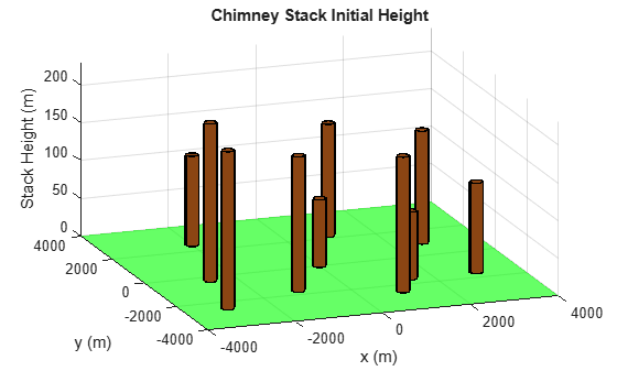
There are two environment related parameters in this problem, the wind speed and direction. Later in this example we will allow these parameters to vary, but for the first problem we will set these parameters to typical values.
% Wind direction in radians
theta0 = 3.996;
% Wind speed in m/s
U0 = 5.64;
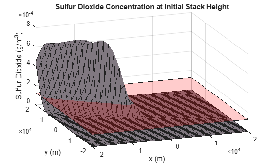
Now let's plot the ground level concentration of sulfur dioxide (SO2) over the entire region R (remember that the plot of chimney stacks was over a smaller region). The SO2 concentration has been calculated with the chimney stacks set to their initial heights.
We can see that the concentration of SO2 varies over the region of interest. There are two features of the Sulfur Dioxide graph of note:
SO2 concentration rises in the top left hand corner of the (x,y) plane
SO2 concentration is approximately zero throughout most of the region
In very simple terms, the first feature is due to the prevailing wind, which is blowing SO2 toward the top left hand corner of the (x,y) plane in this example. The second factor is due to SO2 being transported to the ground via diffusion. This is a slower process compared to the prevailing wind and thus SO2 only reaches ground level in the top left hand corner of the region of interest.
For a more detailed discussion of atmospheric dispersion from chimney stacks, consult the reference cited in the introduction.
The pink plane indicates a SO2 concentration of . This is the legislated maximum for which the Sulfur Dioxide concentration must not exceed in the region R. It can be clearly seen from the graph that the SO2 concentration exceeds the maximum for the initial chimney stack height.
Examine the MATLAB file concSulfurDioxide to see how the sulfur dioxide concentration is calculated.
plotSulfurDioxide(h0, theta0, U0, ...
    "Sulfur Dioxide Concentration at Initial Stack Height");
How fseminf Works
Before we solve the minimal stack height problem, we will outline how fseminf solves a semi-infinite problem. A general semi-infinite programming problem can be stated as:
such that
(Linear inequality constraints)
(Linear equality constraints)
(Nonlinear Inequality Constraints)
(Nonlinear Equality Constraints)
(Bounds)
and
, where for (Nonlinear semi-infinite constraints)
This algorithm allows you to specify constraints for a nonlinear optimization problem that must be satisfied over intervals of an auxiliary variable, . Note that for fseminf, this variable is restricted to be either 1 or 2 dimensional for each semi-infinite constraint.
The function fseminf solves the general semi-infinite problem by starting from an initial value, , and using an iterative procedure to obtain an optimum solution, .
The key component of the algorithm is the handling of the "semi-infinite" constraints, . At it is required that the must be feasible at every value of in the interval . This constraint can be simplified by considering all the local maxima of with respect to in the interval . The original constraint is equivalent to requiring that the value of at each of the above local maxima is feasible.
fseminf calculates an approximation to all the local maximum values of each semi-infinite constraint, . To do this, fseminf first calculates each semi-infinite constraint over a mesh of values. A simple differencing scheme is then used to calculate all the local maximum values of from the evaluated semi-infinite constraint.
As we will see later, you create this mesh in your constraint function. The spacing you should use for each coordinate of the mesh is supplied to your constraint function by fseminf.
At each iteration of the algorithm, the following steps are performed:
Evaluate over a mesh of -values using the current mesh spacing for each -coordinate.
Calculate an approximation to all the local maximum values of using the evaluation of from step 1.
Replace each in the general semi-infinite problem with the set of local maximum values found in steps 1-2. The problem now has a finite number of nonlinear constraints.
fseminfuses the SQP algorithm used byfminconto take one iteration step of the modified problem.Check if any of the SQP algorithm's stopping criteria are met at the new point . If any criteria are met the algorithm terminates; if not,
fseminfcontinues to step 5. For example, if the first order optimality value for the problem defined in step 3 is less than the specified tolerance thenfseminfwill terminate.Update the mesh spacing used in the evaluation of the semi-infinite constraints in step 1.
Writing the Nonlinear Constraint Function
Before we can call fseminf to solve the problem, we need to write a function to evaluate the nonlinear constraints in this problem. The constraint to be implemented is that the ground level Sulfur Dioxide concentration must not exceed at every point in region R.
This is a semi-infinite constraint, and the implementation of the constraint function is explained in this section. For the minimal stack height problem we have implemented the constraint in the airPollutionCon function.
function [ineqnonlin, eqnonlin, K, s] = airPollutionCon(h, s, theta, U)
%AIRPOLLUTIONCON Constraint function for air pollution demo
%
%   [INEQNONLIN, EQNONLIN, K, S] = AIRPOLLUTIONCON(H, S, THETA, U) calculates the
%   constraints for the air pollution Optimization Toolbox (TM) demo. This
%   function first creates a grid of (X, Y) points using the supplied grid
%   spacing, S. The following constraint is then calculated over each point
%   of the grid:
%
%   Sulfur Dioxide concentration at the specified wind direction, THETA and
%   wind speed U <= 1.25e-4 g/m^3
%
%   See also AIRPOLLUTION

%   Copyright 2008-2025 The MathWorks, Inc.

% Initial sampling interval
if nargin < 2 || isnan(s(1,1))
    s = [1000 4000];
end

% Define the grid that the "infinite" constraints will be evaluated over
w1x = -20000:s(1,1):20000;
w1y = -20000:s(1,2):20000;
[t1,t2] = meshgrid(w1x,w1y);

% Maximum allowed sulfur dioxide
maxsul = 1.25e-4;

% Calculate the constraint over the grid
K = concSulfurDioxide(t1, t2, h, theta, U) - maxsul;

% Rescale constraint to make it 0(1)
K = 1e4*K;

% No finite constraints
ineqnonlin = [];
eqnonlin = [];
end
This function illustrates the general structure of a constraint function for a semi-infinite programming problem. In particular, a constraint function for fseminf can be broken up into three parts:
1. Define the initial mesh size for the constraint evaluation
Recall that fseminf evaluates the "semi-infinite" constraints over a mesh as part of the overall calculation of these constraints. When your constraint function is called by fseminf, the mesh spacing you should use is supplied to your function. Fseminf will initially call your constraint function with the mesh spacing, s, set to NaN. This allows you to initialize the mesh size for the constraint evaluation. Here, we have one "infinite" constraint in two "infinite" variables. This means we need to initialize the mesh size to a 1-by-2 matrix, in this case, s = [1000 4000].
2. Define the mesh that will be used for the constraint evaluation
A mesh that will be used for the constraint evaluation needs to be created. The three lines of code following the comment "Define the grid that the "infinite" constraints will be evaluated over" in airPollutionCon can be modified for most 2-d semi-infinite programming problems.
3. Calculate the constraints over the mesh
Once the mesh has been defined, the constraints can be calculated over it. These constraints are then returned to fseminf from the above constraint function.
Note that in this problem, we have also rescaled the constraints so that they vary on a scale which is closer to that of the objective function. This helps fseminf to avoid scaling issues associated with objectives and constraints which vary on disparate scales.
Solve the Optimization Problem
We can now call fseminf to solve the problem. The chimney stacks must all be at least 10m tall and we use the initial stack height specified earlier. Note that the third input argument to fseminf below (1) indicates that there is only one semi-infinite constraint.
lb = 10*ones(size(h0));
[hsopt, sumh, exitflag] = fseminf(@(h)sum(h), h0, 1, ...
    @(h,s) airPollutionCon(h,s,theta0,U0), [], [], [], [], lb);
Local minimum possible. Constraints satisfied. fseminf stopped because the predicted change in the objective function is less than the value of the function tolerance and constraints are satisfied to within the value of the constraint tolerance. <stopping criteria details>
fprintf("\nMinimum computed cumulative height of chimney stacks : %7.2f m\n", sumh);Minimum computed cumulative height of chimney stacks : 3667.19 m
The minimum cumulative height computed by fseminf is considerably higher than the initial total height of the chimney stacks. We will see how the minimum cumulative height changes when parameter uncertainty is added to the problem later in the example. For now, let's plot the chimney stacks at their optimal height.
Examine the MATLAB file plotChimneyStacks to see how the plot was generated.
plotChimneyStacks(hsopt, "Chimney Stack Optimal Height");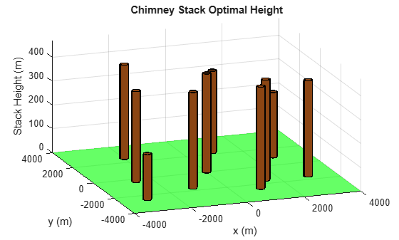
Check the Optimization Results
Recall that fseminf determines that the semi-infinite constraint is satisfied everywhere by ensuring that discretized maxima of the constraint are below the specified bound. We can verify that the semi-infinite constraint is satisfied everywhere by plotting the ground level sulfur dioxide concentration for the optimal stack height.
Note that the sulfur dioxide concentration takes its maximum possible value in the upper left corner of the (x, y) plane, i.e. at x = -20000m, y = 20000m. This point is marked by the blue dot in the figure below and verified by calculating the sulfur dioxide concentration at this point.
Examine the MATLAB file plotSulfurDioxide to see how the plots was generated.
titleStr = "Optimal Sulfur Dioxide Concentration and its maximum (blue)";
xMaxSD = [-20000 20000];
plotSulfurDioxide(hsopt, theta0, U0, titleStr, xMaxSD);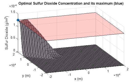
SO2Max = concSulfurDioxide(-20000, 20000, hsopt, theta0, U0);
fprintf("Sulfur Dioxide Concentration at x = -20000m, y = 20000m : %e g/m^3\n", SO2Max);
Sulfur Dioxide Concentration at x = -20000m, y = 20000m : 1.250000e-04 g/m^3
Considering Uncertainty in the Environmental Factors
The sulfur dioxide concentration depends on several environmental factors which were held at fixed values in the above problem. Two of the environmental factors are wind speed and wind direction. See the reference cited in the introduction for a more detailed discussion of all the problem parameters.
We can investigate the change in behavior for the system with respect to the wind speed and direction. In this section of the example, we want to make sure that the sulfur dioxide limits are satisfied even if the wind direction changes from 3.82 rad to 4.18 rad and mean wind speed varies between 5 and 6.2 m/s.
We need to implement a semi-infinite constraint to ensure that the sulfur dioxide concentration does not exceed the limit in region R. This constraint is required to be feasible for all pairs of wind speed and direction.
Such a constraint will have four "infinite" variables (wind speed and direction and the x-y coordinates of the ground). However, any semi-infinite constraint supplied to fseminf can have no more than two "infinite" variables.
To implement this constraint in a suitable form for fseminf, we recall the SO2 concentration at the optimum stack height in the previous problem. In particular, the SO2 concentration takes its maximum possible value at x = -20000m, y = 20000m. To reduce the number of "infinite" variables, we will assume that the SO2 concentration will also take its maximum value at this point when uncertainty is present. We then require that SO2 concentration at this point is below for all pairs of wind speed and direction.
This means that the "infinite" variables for this problem are wind speed and direction. To see how this constraint has been implemented, inspect the MATLAB function uncertainAirPollutionCon.
function [ineqnonlin, eqnonlin, K, s] = uncertainAirPollutionCon(h, s)
%UNCERTAINAIRPOLLUTIONCON Constraint function for air pollution demo
%
%   [INEQNONLIN, EQNONLIN, K, S] = UNCERTAINAIRPOLLUTIONCON(H, S) calculates the
%   constraints for the fseminf Optimization Toolbox (TM) demo. This
%   function first creates a grid of wind speed/direction points using the
%   supplied grid spacing, S. The following constraint is then calculated
%   over each point of the grid:
%
%   Sulfur Dioxide concentration at x = -20000m, y = 20000m <= 1.25e-4
%   g/m^3
%
%   See also AIRPOLLUTIONCON, AIRPOLLUTION

%   Copyright 2008-2025 The MathWorks, Inc.

% Maximum allowed sulphur dioxide
maxsul = 1.25e-4;

% Initial sampling interval
if nargin < 2 || isnan(s(1,1))
    s = [0.02 0.04];
end

% Define the grid that the "infinite" constraints will be evaluated over
w1x = 3.82:s(1,1):4.18; % Wind direction
w1y = 5.0:s(1,2):6.2;   % Wind speed
[t1,t2] = meshgrid(w1x,w1y);

% We assume the maximum SO2 concentration is at [x, y] = [-20000, 20000]
% for all wind speed/direction pairs. We evaluate the SO2 constraint over
% the [theta, U] grid at this point.
K = concSulfurDioxide(-20000, 20000, h, t1, t2) - maxsul;

% Rescale constraint to make it 0(1)
K = 1e4*K;

% No finite constraints
ineqnonlin = [];
eqnonlin = [];
end
This constraint function can be divided into same three sections as before:
1. Define the initial mesh size for the constraint evaluation
The code following the comment "Initial sampling interval" initializes the mesh size.
2. Define the mesh that will be used for the constraint evaluation
The next section of code creates a mesh (now in wind speed and direction) using a similar construction to that used in the initial problem.
3. Calculate the constraints over the mesh
The remainder of the code calculates the SO2 concentration at each point of the wind speed/direction mesh. These constraints are then returned to fseminf from the above constraint function.
We can now call fseminf to solve the stack height problem considering uncertainty in the environmental factors.
[hsopt2, sumh2, exitflag2] = fseminf(@(h)sum(h), h0, 1, ...
    @uncertainAirPollutionCon, [], [], [], [], lb);
Local minimum possible. Constraints satisfied. fseminf stopped because the predicted change in the objective function is less than the value of the function tolerance and constraints are satisfied to within the value of the constraint tolerance. <stopping criteria details>
fprintf("\nMinimal computed cumulative height of chimney stacks with uncertainty: %7.2f m\n", sumh2);Minimal computed cumulative height of chimney stacks with uncertainty: 3812.08 m
We can now look at the difference between the minimum computed cumulative stack height for the problem with and without parameter uncertainty. You should be able to see that the minimum cumulative height increases when uncertainty is added to the problem. This expected increase in height allows the SO2 concentration to remain below the legislated maximum for all wind speed/direction pairs in the specified range.
We can check that the sulfur dioxide concentration does not exceed the limit over the region of interest via inspection of a sulfur dioxide plot. For a given (x, y) point, we plot the maximum SO2 concentration for the wind speed and direction in the stated ranges. Note that we have zoomed in on the upper left corner of the X-Y plane.
titleStr = "Optimal Sulfur Dioxide Concentration under Uncertainty";
thetaRange = 3.82:0.02:4.18;
URange = 5:0.2:6.2;
XRange = [-20000,-15000];
YRange = [15000,20000];
plotSulfurDioxideUncertain(hsopt2, thetaRange, URange, XRange, YRange, titleStr);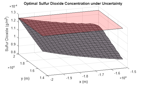
We finally plot the chimney stacks at their optimal height when there is uncertainty in the problem definition.
plotChimneyStacks(hsopt2, "Chimney Stack Optimal Height under Uncertainty");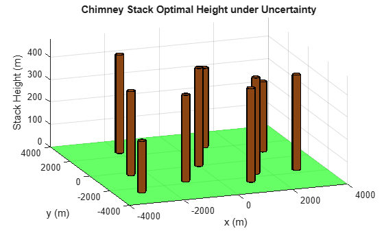
There are many options available for the semi-infinite programming algorithm, fseminf. Consult the Optimization Toolbox™ User's Guide for details, in the Using Optimization Toolbox Solvers chapter, under Constrained Nonlinear Optimization: fseminf Problem Formulation and Algorithm.