Banana Function Minimization

R2026b

This example shows how to minimize Rosenbrock's "banana function":

$$f(x)=100(x(2)-x(1{)}^2{)}^2+(1-x(1){)}^2.$$

$$f(x)$$ is called the banana function because of its curvature around the origin. It is notorious in optimization examples because of the slow convergence most methods exhibit when trying to solve this problem.

$$f(x)$$ has a unique minimum at the point $$x=[1,1]$$ where $$f(x)=0$$. This example shows a number of ways to minimize $$f(x)$$ starting at the point $$x0=[-1.9,2]$$.

Optimization Without Derivatives

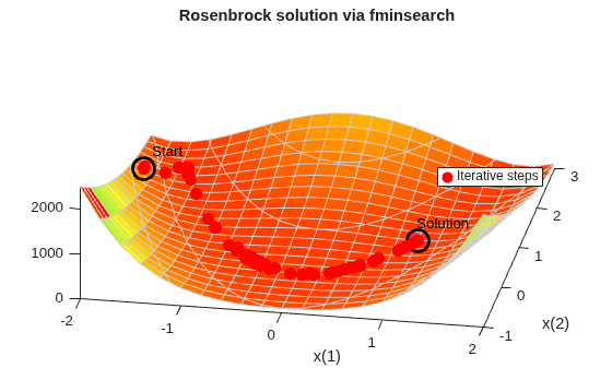
The fminsearch function finds a minimum for a problem without constraints. It uses an algorithm that does not estimate any derivatives of the objective function. Rather, it uses a geometric search method described in fminsearch Algorithm.

Minimize the banana function using fminsearch. Include an output function to report the sequence of iterations.

fun = @(x)(100*(x(2) - x(1)^2)^2 + (1 - x(1))^2);
options = optimset(OutputFcn=@bananaout,Display="off");
x0 = [-1.9,2];
[x,fval,eflag,output] = fminsearch(fun,x0,options);
title("Rosenbrock solution via fminsearch")

Fcount = output.funcCount;
disp("Number of function evaluations for fminsearch is " + string(Fcount))

Number of function evaluations for fminsearch is 210

disp("Number of solver iterations for fminsearch is " + string(output.iterations))

Number of solver iterations for fminsearch is 114

Optimization with Estimated Derivatives

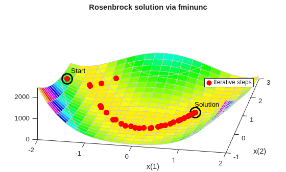
The fminunc function finds a minimum for a problem without constraints. It uses a derivative-based algorithm. The algorithm attempts to estimate not only the first derivative of the objective function, but also the matrix of second derivatives. fminunc is usually more efficient than fminsearch.

Minimize the banana function using fminunc.

options = optimoptions("fminunc",Display="off",...
    OutputFcn=@bananaout,Algorithm="quasi-newton");
[x,fval,eflag,output] = fminunc(fun,x0,options);
title("Rosenbrock solution via fminunc")

Fcount = output.funcCount;
disp("Number of function evaluations for fminunc is " + string(Fcount))

Number of function evaluations for fminunc is 150

disp("Number of solver iterations for fminunc is "+ string(output.iterations))

Number of solver iterations for fminunc is 34

Optimization with Steepest Descent

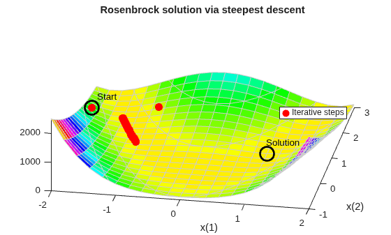
If you attempt to minimize the banana function using a steepest descent algorithm, the high curvature of the problem makes the solution process very slow.

You can run fminunc with the steepest descent algorithm by setting the hidden HessUpdate option to the value "steepdesc" for the "quasi-newton" algorithm. Set a larger-than-default maximum number of function evaluations, because the solver does not find the solution quickly. In this case, the solver does not find the solution even after 600 function evaluations.

options = optimoptions(options,HessUpdate="steepdesc",...
    MaxFunctionEvaluations=600);
[x,fval,eflag,output] = fminunc(fun,x0,options);
title("Rosenbrock solution via steepest descent")

Fcount = output.funcCount;
disp("Number of function evaluations for steepest descent is "...
    + string(Fcount))

Number of function evaluations for steepest descent is 600

disp("Number of solver iterations for steepest descent is "...
    + string(output.iterations))

Number of solver iterations for steepest descent is 45

Optimization with Analytic Gradient

If you provide a gradient, fminunc solves the optimization using fewer function evaluations. When you provide a gradient, you can use the "trust-region" algorithm, which is often faster and uses less memory than the "quasi-newton" algorithm. Reset the HessUpdate and MaxFunctionEvaluations options to their default values.

grad = @(x)[-400*(x(2) - x(1)^2)*x(1) - 2*(1 - x(1));
            200*(x(2) - x(1)^2)];
fungrad = @(x)deal(fun(x),grad(x));
options = resetoptions(options,{"HessUpdate","MaxFunctionEvaluations"});
options = optimoptions(options,SpecifyObjectiveGradient=true,...
    Algorithm="trust-region");
[x,fval,eflag,output] = fminunc(fungrad,x0,options);
title("Rosenbrock solution via fminunc with gradient")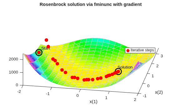

Fcount = output.funcCount;
disp("Number of function evaluations for fminunc with gradient is "...
    + string(Fcount))

Number of function evaluations for fminunc with gradient is 32

disp("Number of solver iterations for fminunc with gradient is "...
    + string(output.iterations))

Number of solver iterations for fminunc with gradient is 31

Optimization with Analytic Hessian

If you provide a Hessian (matrix of second derivatives), fminunc can solve the optimization using even fewer function evaluations. For this problem the results are the same with or without the Hessian.

hess = @(x)[1200*x(1)^2 - 400*x(2) + 2, -400*x(1);
            -400*x(1), 200];
fungradhess = @(x)deal(fun(x),grad(x),hess(x));
options.HessianFcn = "objective";
[x,fval,eflag,output] = fminunc(fungradhess,x0,options);
title("Rosenbrock solution via fminunc with Hessian")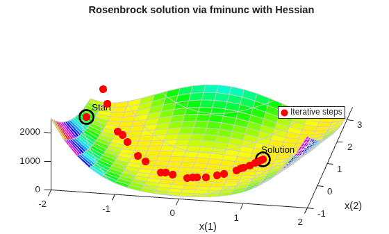

Fcount = output.funcCount;
disp("Number of function evaluations for fminunc with gradient and Hessian is "...
    + string(Fcount))

Number of function evaluations for fminunc with gradient and Hessian is 32

disp("Number of solver iterations for fminunc with gradient and Hessian is " + string(output.iterations))

Number of solver iterations for fminunc with gradient and Hessian is 31

Optimization with a Least Squares Solver

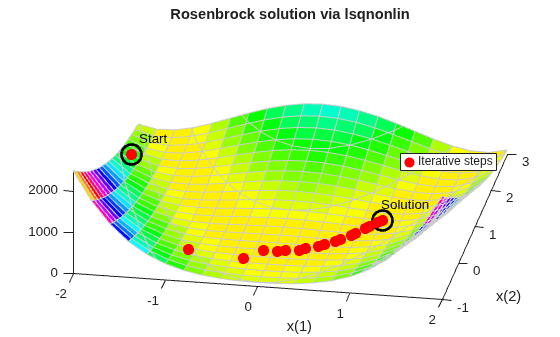
The recommended solver for a nonlinear sum of squares is lsqnonlin. This solver is even more efficient than fminunc without a gradient for this special class of problems. To use lsqnonlin, do not write your objective as a sum of squares. Instead, write the underlying vector that lsqnonlin internally squares and sums.

options = optimoptions("lsqnonlin",Display="off",OutputFcn=@bananaout);
vfun = @(x)[10*(x(2) - x(1)^2),1 - x(1)];
[x,resnorm,residual,eflag,output] = lsqnonlin(vfun,x0,[],[],options);
title("Rosenbrock solution via lsqnonlin")

Fcount = output.funcCount;
disp("Number of function evaluations for lsqnonlin is "...
    + string(Fcount))

Number of function evaluations for lsqnonlin is 87

disp("Number of solver iterations for lsqnonlin is " + string(output.iterations))

Number of solver iterations for lsqnonlin is 28

Optimization with a Least Squares Solver and Jacobian

As in the minimization using a gradient for fminunc, lsqnonlin can use derivative information to lower the number of function evaluations. Provide the Jacobian of the nonlinear objective function vector and run the optimization again.

jac = @(x)[-20*x(1),10;
           -1,0];
vfunjac = @(x)deal(vfun(x),jac(x));
options.SpecifyObjectiveGradient = true;
[x,resnorm,residual,eflag,output] = lsqnonlin(vfunjac,x0,[],[],options);
title("Rosenbrock solution via lsqnonlin with Jacobian")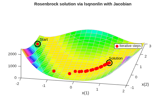

Fcount = output.funcCount;
disp("Number of function evaluations for lsqnonlin with Jacobian is "...
    + string(Fcount))

Number of function evaluations for lsqnonlin with Jacobian is 29

disp("Number of solver iterations for lsqnonlin with Jacobian is "...
    + string(output.iterations))

Number of solver iterations for lsqnonlin with Jacobian is 28