Helmholtz Equation on Disk with Square Hole
This example shows how to solve a Helmholtz equation using the general PDEModel container and the solvepde function. For the electromagnetic workflow that uses ElectromagneticModel and familiar domain-specific language, see Scattering Problem.
Solve a simple scattering problem, where you compute the waves reflected by a square object illuminated by incident waves that are coming from the left. For this problem, assume an infinite horizontal membrane subjected to small vertical displacements U. The membrane is fixed at the object boundary. The medium is homogeneous, and the phase velocity (propagation speed) of a wave, α, is constant. The wave equation is
The solution U is the sum of the incident wave V and the reflected wave R:
When the illumination is harmonic in time, you can compute the field by solving a single steady problem. Assume that the incident wave is a plane wave traveling in the -x direction:
The reflected wave can be decomposed into spatial and time components:
Now you can rewrite the wave equation as the Helmholtz equation for the spatial component of the reflected wave with the wave number :
The Dirichlet boundary condition for the boundary of the object is U = 0, or in terms of the incident and reflected waves, R = -V. For the time-harmonic solution and the incident wave traveling in the -x direction, you can write this boundary condition as follows:
The reflected wave R travels outward from the object. The condition at the outer computational boundary must allow waves to pass without reflection. Such conditions are usually called nonreflecting. As approaches infinity, R approximately satisfies the one-way wave equation
This equation considers only the waves moving in the positive ξ-direction. Here, ξ is the radial distance from the object. With the time-harmonic solution, this equation turns into the generalized Neumann boundary condition
To solve the scattering problem using the programmatic workflow, first create a PDE model with a single dependent variable.
numberOfPDE = 1;
model = createpde(numberOfPDE);
Specify the variables that define the problem:
g: A geometry specification function. For more information, see the documentation section Parameterized Function for 2-D Geometry Creation and the code forscatterg.m.k,c,a,f: The coefficients and inhomogeneous term.
g = @scatterg;
k = 60;
c = 1;
a = -k^2;
f = 0;
Convert the geometry and append it to the model.
geometryFromEdges(model,g);
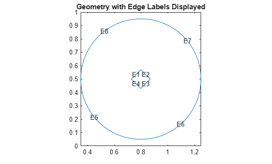
Plot the geometry and display the edge labels for use in the boundary condition definition.
figure;
pdegplot(model,EdgeLabels="on");
axis equal
title("Geometry with Edge Labels Displayed")
ylim([0,1])
Apply the boundary conditions.
bOuter = applyBoundaryCondition(model,"neumann", ...
                                Edge=(5:8),g=0,q=-60i);
innerBCFunc = @(loc,state)-exp(-1i*k*loc.x);
bInner = applyBoundaryCondition(model,"dirichlet", ...
                                Edge=(1:4),u=innerBCFunc);
Specify the coefficients.
specifyCoefficients(model,m=0,d=0,c=c,a=a,f=f);
Generate a mesh.
generateMesh(model,Hmax=0.02);
figure
pdemesh(model);
axis equal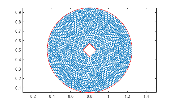
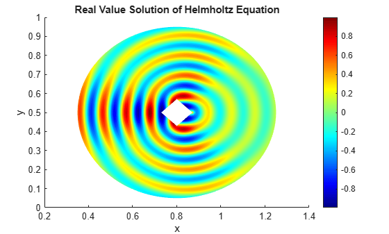
Solve for the complex amplitude. The real part of vector u stores an approximation to a real value solution of the Helmholtz equation.
result = solvepde(model);
u = result.NodalSolution;
Plot the solution.
figure
pdeplot(model,XYData=real(u),Mesh="off");
colormap(jet)
xlabel("x")
ylabel("y")
title("Real Value Solution of Helmholtz Equation")
Using the solution to the Helmholtz equation, create an animation showing the corresponding solution to the time-dependent wave equation.
figure
m = 10;
maxu = max(abs(u));
for j = 1:m
    uu = real(exp(-j*2*pi/m*sqrt(-1))*u);
    pdeplot(model,XYData=uu,ColorBar="off",Mesh="off");
    colormap(jet)
    axis tight
    ax = gca;
    ax.DataAspectRatio = [1 1 1];
    axis off
    M(j) = getframe;
end
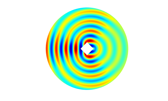
To play the movie, use the movie(M) command.