plotResponse

System object: phased.HeterogeneousULA
Namespace: phased

Plot response pattern of array

Syntax

plotResponse(H,FREQ,V)
plotResponse(H,FREQ,V,Name,Value)
hPlot = plotResponse(___)


Description

plotResponse(H,FREQ,V) plots the array response pattern along the azimuth cut, where the elevation angle is 0. The operating frequency is specified in FREQ. The propagation speed is specified in V.

plotResponse(H,FREQ,V,Name,Value) plots the array response with additional options specified by one or more Name,Value pair arguments.

hPlot = plotResponse(___) returns handles of the lines or surface in the figure window, using any of the input arguments in the previous syntaxes.

Input Arguments

H	Array object
FREQ	Operating frequency in Hertz specified as a scalar or 1-by-K row vector. Values must lie within the range specified by a property of H. That property is named FrequencyRange or FrequencyVector, depending on the type of element in the array. The element has no response at frequencies outside that range. If you set the 'RespCut' property of H to '3D', FREQ must be a scalar. When FREQ is a row vector, plotResponse draws multiple frequency responses on the same axes.
V	Propagation speed in meters per second.

Name-Value Arguments

Specify optional pairs of arguments as Name1=Value1,...,NameN=ValueN, where Name is the argument name and Value is the corresponding value. Name-value arguments must appear after other arguments, but the order of the pairs does not matter.

Before R2021a, use commas to separate each name and value, and enclose Name in quotes.

CutAngle	Cut angle as a scalar. This argument is applicable only when RespCut is 'Az' or 'El'. If RespCut is 'Az', CutAngle must be between –90 and 90. If RespCut is 'El', CutAngle must be between –180 and 180. Default: 0
Format	Format of the plot, using one of 'Line', 'Polar', or 'UV'. If you set Format to 'UV', FREQ must be a scalar. Default: 'Line'
NormalizeResponse	Set this value to true to normalize the response pattern. Set this value to false to plot the response pattern without normalizing it. This parameter is not applicable when you set the Unit parameter value to 'dbi'. Default: true
OverlayFreq	Set this value to true to overlay pattern cuts in a 2-D line plot. Set this value to false to plot pattern cuts against frequency in a 3-D waterfall plot. If this value is false, FREQ must be a vector with at least two entries. This parameter applies only when Format is not 'Polar' and RespCut is not '3D'. Default: true
Polarization	Specify the polarization options for plotting the array response pattern. The allowable values are |'None' | 'Combined' | 'H' | 'V' | where 'None' specifies plotting a nonpolarized response pattern 'Combined' specifies plotting a combined polarization response pattern 'H' specifies plotting the horizontal polarization response pattern 'V' specifies plotting the vertical polarization response pattern For arrays that do not support polarization, the only allowed value is 'None'. This parameter is not applicable when you set the Unit parameter value to 'dbi'. Default: 'None'
RespCut	Cut of the response. Valid values depend on Format, as follows: If Format is 'Line' or 'Polar', the valid values of RespCut are 'Az', 'El', and '3D'. The default is 'Az'. If Format is 'UV', the valid values of RespCut are 'U' and '3D'. The default is 'U'. If you set RespCut to '3D', FREQ must be a scalar.
Unit	The unit of the plot. Valid values are 'db', 'mag', 'pow', or 'dbi'. This parameter determines the type of plot that is produced. Unit value Plot type db power pattern in dB scale mag field pattern pow power pattern dbi directivity Default: 'db'
Weights	Weight values applied to the array, specified as a length-N column vector or N-by-M matrix. The dimension N is the number of elements in the array. The interpretation of M depends upon whether the input argument FREQ is a scalar or row vector. Weights Dimensions FREQ Dimension Purpose N-by-1 column vector Scalar or 1-by-M row vector Apply one set of weights for the same single frequency or all M frequencies. N-by-M matrix Scalar Apply all of the M different columns in Weights for the same single frequency. 1-by-M row vector Apply each of the M different columns in Weights for the corresponding frequency in FREQ.
AzimuthAngles	Azimuth angles for plotting array response, specified as a row vector. The AzimuthAngles parameter sets the display range and resolution of azimuth angles for visualizing the radiation pattern. This parameter is allowed only when the RespCut parameter is set to 'Az' or '3D' and the Format parameter is set to 'Line' or 'Polar'. The values of azimuth angles should lie between –180° and 180° and must be in nondecreasing order. When you set the RespCut parameter to '3D', you can set the AzimuthAngles and ElevationAngles parameters simultaneously. Default: [-180:180]
ElevationAngles	Elevation angles for plotting array response, specified as a row vector. The ElevationAngles parameter sets the display range and resolution of elevation angles for visualizing the radiation pattern. This parameter is allowed only when the RespCut parameter is set to 'El' or '3D' and the Format parameter is set to 'Line' or 'Polar'. The values of elevation angles should lie between –90° and 90° and must be in nondecreasing order. When yous set the RespCut parameter to '3D', you can set the ElevationAngles and AzimuthAngles parameters simultaneously. Default: [-90:90]
UGrid	U coordinate values for plotting array response, specified as a row vector. The UGrid parameter sets the display range and resolution of the U coordinates for visualizing the radiation pattern in U/V space. This parameter is allowed only when the Format parameter is set to 'UV' and the RespCut parameter is set to 'U' or '3D'. The values of UGrid should be between –1 and 1 and should be specified in nondecreasing order. You can set the UGrid and VGrid parameters simultaneously. Default: [-1:0.01:1]
VGrid	V coordinate values for plotting array response, specified as a row vector. The VGrid parameter sets the display range and resolution of the V coordinates for visualizing the radiation pattern in U/V space. This parameter is allowed only when the Format parameter is set to 'UV' and the RespCut parameter is set to '3D'. The values of VGrid should be between –1 and 1 and should be specified in nondecreasing order. You can set VGrid and UGrid parameters simultaneously. Default: [-1:0.01:1]

Examples

Line Plot Showing Multiple Frequencies

Using a line plot, show the azimuth cut response of a 5-element heterogeneous uniform linear array along 0 degrees elevation. The plot shows the responses at operating frequencies of 200 MHz and 400 MHz.

Construct the array from z-directed and y-directed short dipole antenna elements.

sElement1 = phased.ShortDipoleAntennaElement(...
    'FrequencyRange',[2e8 5e8],...
    'AxisDirection','Z');
sElement2 = phased.ShortDipoleAntennaElement(...
    'FrequencyRange',[2e8 5e8],...
    'AxisDirection','Y');
sArray = phased.HeterogeneousULA(...
    'ElementSet',{sElement1,sElement2},...
    'ElementIndices',[1 2 2 2 1]);

Plot the response.

fc = [3e8 4e8];
c = physconst('LightSpeed');
plotResponse(sArray,fc,c);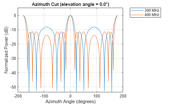

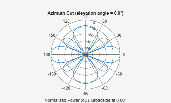
Plot Response and Directivity for 5-Element Array

Construct a 5-element heterogeneous ULA of short-dipole antenna elements. Using the plotResponse method, plot the array's azimuth response in polar format. Assume each element's operating frequency spans 200-500 MHz and the wave propagation speed is the speed of light.

sElement1 = phased.ShortDipoleAntennaElement(...
    'FrequencyRange',[2e8 5e8],...
    'AxisDirection','Z');
sElement2 = phased.ShortDipoleAntennaElement(...
    'FrequencyRange',[2e8 5e8],...
    'AxisDirection','Y');
sArray = phased.HeterogeneousULA(...
    'ElementSet',{sElement1,sElement2},...
    'ElementIndices',[1 2 2 2 1]);

Plot the response at 300 MHz.

fc = 3e8;
c = physconst('LightSpeed');
plotResponse(sArray,fc,c,'RespCut','Az','Format','Polar');

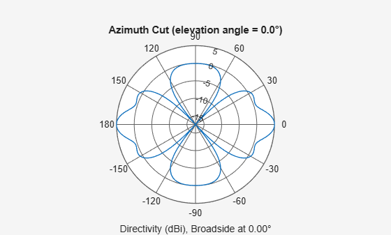
Plot the directivity of the array at 300 MHz.

plotResponse(sArray,fc,c,'RespCut','Az','Format','Polar',...
    'Unit','dbi');

Plot Response for 9-Element Array with Two Weight Sets

Construct a 9-element heterogeneous ULA of short-dipole antenna elements having different orientations. Assume each element response is in the frequency range 200-500 MHz. Using the plotResponse method, plot the array's azimuth response in polar format. Use the Weights parameter to set two different sets of tapering weights: a uniform tapering and a Taylor tapering. Use the AzimuthAngles parameter to restrict the display range from -45 to 45 degrees in 0.1 degree increments.

Construct the array.

sElement1 = phased.ShortDipoleAntennaElement(...
    'FrequencyRange',[2e8 5e8],...
    'AxisDirection','Z');
sElement2 = phased.ShortDipoleAntennaElement(...
    'FrequencyRange',[2e8 5e8],...
    'AxisDirection','Y');
sArray = phased.HeterogeneousULA(...
    'ElementSet',{sElement1,sElement2},...
    'ElementIndices',[1 1 2 2 2 2 2 1 1]);

Plot the response at 300 MHz.

fc = 3e8;
wts1 = ones(9,1);
wts2 = taylorwin(9);
c = physconst('LightSpeed');
plotResponse(sArray,fc,c,'RespCut','Az',...
    'AzimuthAngles',[-45:0.1:45],...
    'Weights',[wts1,wts2]);

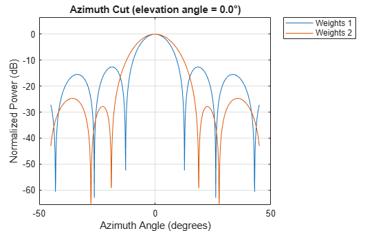
As expected, the tapered weighting broadens the mainlobe and reduces the sidelobes.