polloss
Polarization loss
Syntax
Description
rho = polloss(fv_tr,fv_rcv)fv_tr, and the polarization
of the receiving antenna, fv_rcv. The field
vector lies in a plane orthogonal to the direction of propagation
from the transmitter to the receiver. The transmitted field is represented
as a 2-by-1 column vector [Eh;Ev]. In this vector, Eh and Ev are
the field’s horizontal and vertical linear polarization components
with respect to the transmitter’s local coordinate system.
The receiving antenna’s polarization is specified by a 2-by-1
column vector, fv_rcv. You can also specify this
polarization in the form of [Eh;Ev] with respect
to the receiving antenna’s local coordinate system. In this
syntax, both local coordinate axes align with the global coordinate
system.
rho = polloss(fv_tr,fv_rcv,pos_rcv,axes_rcv)axes_rcv.
These axes define the receiver's local coordinate system as a 3-by-3
matrix. The first column gives the x-axis of the
local system with respect to the global coordinate system. The second
and third columns give the y and z axes,
respectively. This syntax can use any of the input arguments in the
previous syntaxes.
rho = polloss(fv_tr,fv_rcv,pos_rcv,axes_rcv,pos_tr,axes_tr)axes_tr. These
axes define the transmitter's local coordinate system as a 3-by-3
matrix. The first column gives the x-axis of the
local system with respect to the global coordinate system. The second
and third columns give the y and z axes,
respectively. This syntax can use any of the input arguments in the
previous syntaxes.
Examples
Begin with a 45° polarized transmitted field and a receiver that is horizontally polarized. By default, the transmitter and receiver local axes coincide with the global coordinate system. Compute the polarization loss in dB.
fv_tr = [1;1];
fv_rcv = [1;0];
rho = polloss(fv_tr,fv_rcv)
rho =
3.0103
The loss is 3 dB as expected because only half the power of the field matches to the receive antenna polarization.
Begin with identical transmitter and receiver polarizations. Place the receiver at a position 100 meters along the y-axis. The transmitter is at the origin (its default position) and both local coordinate axes coincide with the global coordinate system (by default). First, compute the polarization loss. Then, move the receiver 100 meters along the x-axis, and compute the polarization loss again.
fv_tr = [1;0];
fv_rcv = [1;0];
pos_rcv = [0;100;0];
rho(1) = polloss(fv_tr,fv_rcv,pos_rcv);
pos_rcv = [100;100;0];
rho(2) = polloss(fv_tr,fv_rcv,pos_rcv)
rho = 1×2

     0     0
No polarization loss occurs at either position. The spherical basis vectors of each antenna are parallel to other antenna and the polarization vectors are the same.
Start with identical transmitter and receiver polarizations. Put the receiver at a position 100 meters along the y-axis. The transmitter is at the origin (default) and both local coordinate axes coincide with the global coordinate system (default). Compute the loss, and then rotate the receiver 30° around the y-axis. This rotation changes the azimuth and elevation of the transmitter with respect to the receiver and, therefore, the direction of polarization.
fv_tr = [1;0];
fv_rcv = [1;0];
pos_rcv = [0;100;0];
ax_rcv = azelaxes(0,0);
rho(1) = polloss(fv_tr,fv_rcv,pos_rcv,ax_rcv);
ax_rcv = roty(30)*ax_rcv;
rho(2) = polloss(fv_tr,fv_rcv,pos_rcv,ax_rcv)
rho = 1×2

         0    1.2494
The receiver polarization vector remains unchanged. However, rotating the local coordinate system changes the direction of the field of the receiving antenna polarization with respect to global coordinates. This change results in a 1.2 dB loss.
Start with identical transmitter and receiver polarizations. Put the receiver at a position 100 meters along the y-axis. The transmitter is at the origin (default) and both local coordinate axes coincide with the global coordinate system (default). First, compute the polarization loss. Then, move the transmitter 100 meters along the x-axis and 100 meters along the y-axis, and compute the polarization loss again.
fv_tr = [1;0];
fv_rcv = [1;0];
pos_rcv = [0;100;0];
ax_rcv = azelaxes(0,0);
pos_tr = [0;0;0];
rho(1) = polloss(fv_tr,fv_rcv,pos_rcv,ax_rcv,pos_tr);
pos_tr = [100;100;0];
rho(2) = polloss(fv_tr,fv_rcv,pos_rcv,ax_rcv,pos_tr)
rho = 1×2

     0     0
There is no polarization loss at either position because the spherical basis vectors of each antenna are parallel to their counterparts and the polarization vectors are the same.
Specifying identical transmitter and receiver polarizations, plot the loss as the local receiving antenna axes rotate around the -axis.
fv_tr = [1;0];
fv_rcv = [1;0];
The position of the transmitting antenna is at the origin and its local axes align with the global coordinate system. The position of the receiving antenna is 100 meters along the global -axis. However, its local -axis points towards the transmitting antenna.
pos_tr = [0;0;0];
axes_tr = azelaxes(0,0);
pos_rcv = [100;0;0];
axes_rcv0 = rotz(180)*azelaxes(0,0);
Rotate the receiving antenna around its local -axis in one-degree increments. Compute the loss for each angle.
angles = [0:1:359];
n = size(angles,2);
rho = zeros(1,n); % Initialize space
for k = 1:n
    axes_rcv = rotx(angles(k))*axes_rcv0;
    rho(k) = polloss(fv_tr,fv_rcv,pos_tr,axes_tr,...
        pos_rcv,axes_rcv);
end
Plot the polarization loss.
hp = plot(angles,rho);
hax = hp.Parent;
hax.XLim = [0,360];
xticks = (0:(n-1))*45;
hax.XTick = xticks;
grid;
title('Polarization loss versus receiving antenna rotation')
xlabel('Rotation angle (degrees)');
ylabel('Loss (dB)');
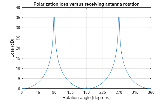
The angle-loss plot shows nulls (Inf dB) at 90 degrees and 270 degrees where the polarizations are orthogonal.
Input Arguments
Output Arguments
More About
Loss occurs when a receiver is not matched to the polarization of an incident electromagnetic field.
In the case of the polarization of a field emitted by a transmitting antenna, first, look at the far zone of the transmitting antenna, as shown in the following figure. At this location―which is the location of the receiving antenna―the electromagnetic field is orthogonal to the direction from transmitter to receiver.
You can represent the transmitted electromagnetic field, fv_tr,
by the components of a vector with respect to a spherical basis of
the transmitter’s local coordinate system. The orientation
of this basis depends on its direction from the origin. The direction
is specified by the azimuth and elevation of the receiving antenna
with respect to the transmitter’s local coordinate system.
Then, the transmitter’s polarization, in terms of the spherical
basis vectors of the transmitter’s local coordinate system,
is
In the same manner, the receiver’s polarization vector, fv_rcv,
is defined with respect to a spherical basis in the receiver’s
local coordinate system. Now, the azimuth and elevation specify the
transmitter’s position with respect to the receiver’s
local coordinate system. You can write the receiving antennas polarization
in terms of the spherical basis vectors of the receiver’s local
coordinate system:
This figure shows the construction of the different transmitter and receiver local coordinate systems. It also shows the spherical basis vectors with which to write the field components.

The polarization loss is the projection (or dot product) of the normalized transmitted field vector onto the normalized receiver polarization vector. Notice that the loss occurs because of the mismatch in direction of the two vectors not in their magnitudes. Because the vectors are defined in different coordinate systems, they must be converted to the global coordinate system in order to form the projection. The polarization loss is defined by:
References
[1] Mott, H. Antennas for Radar and Communications.John Wiley & Sons, 1992.
Extended Capabilities
Version History
Introduced in R2013a