Underwater Target Detection with an Active Sonar System
R2026bThis example explains how to simulate an active monostatic sonar scenario with two targets. The sonar system consists of an isotropic projector array and a single hydrophone element. The projector array is spherical in shape. The backscattered signals are received by the hydrophone. The received signals include both direct and multipath contributions.
Underwater Environment
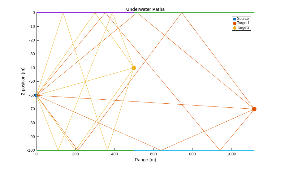
Multiple propagation paths are present between the sound source and target in a shallow water environment. In this example, five paths are assumed in a channel with a depth of 100 meters and a constant sound speed of 1520 m/s. Use a bottom loss of 0.5 dB in order to highlight the effects of the multiple paths.
Define the properties of the underwater environment, including the channel depth, the number of propagation paths, the propagation speed, and the bottom loss.
numPaths = 5;
propSpeed = 1520;
channelDepth = 100;

isopath{1} = phased.IsoSpeedUnderwaterPaths(...
          'ChannelDepth',channelDepth,...
          'NumPathsSource','Property',...
          'NumPaths',numPaths,...
          'PropagationSpeed',propSpeed,...
          'BottomLoss',0.5,...
          'TwoWayPropagation',true);

isopath{2} = phased.IsoSpeedUnderwaterPaths(...
          'ChannelDepth',channelDepth,...
          'NumPathsSource','Property',...
          'NumPaths',numPaths,...
          'PropagationSpeed',propSpeed,...
          'BottomLoss',0.5,...
          'TwoWayPropagation',true);
Next, create a multipath channel for each target. The multipath channel propagates the waveform along the multiple paths. This two-step process is analogous to designing a filter and using the resulting coefficients to filter a signal.
fc = 20e3;   % Operating frequency (Hz)

channel{1} = phased.MultipathChannel(...
          'OperatingFrequency',fc);

channel{2} = phased.MultipathChannel(...
          'OperatingFrequency',fc);
Sonar Targets
The scenario has two targets. The first target is more distant but has a larger target strength, and the second is closer but has a smaller target strength. Both targets are isotropic and stationary with respect to the sonar system.
tgt{1} = phased.BackscatterSonarTarget(...
    'TSPattern',-5*ones(181,361));

tgt{2} = phased.BackscatterSonarTarget(...
    'TSPattern',-15*ones(181,361));

tgtplat{1} = phased.Platform(...
    'InitialPosition',[500; 1000; -70],'Velocity',[0; 0; 0]);

tgtplat{2} = phased.Platform(...
    'InitialPosition',[500; 0; -40],'Velocity',[0; 0; 0]);
The target positions, along with the channel properties, determine the underwater paths along which the signals propagate. Plot the paths between the sonar system and each target. Note that the z-coordinate determines depth, with zero corresponding to the top surface of the channel, and the distance in the x-y plane is plotted as the range between the source and target.
helperPlotPaths([0;0;-60],[500 500; 1000 0; -70 -40], ...
  channelDepth,numPaths)
Transmitter and Receiver
Transmitted Waveform
Next, specify a rectangular waveform to transmit to the targets. The maximum target range and desired range resolution define the properties of the waveform.
maxRange = 5000;                         % Maximum unambiguous range
rangeRes = 10;                           % Required range resolution
prf = propSpeed/(2*maxRange);            % Pulse repetition frequency
pulse_width = 2*rangeRes/propSpeed;      % Pulse width
pulse_bw = 1/pulse_width;                % Pulse bandwidth
fs = 2*pulse_bw;                         % Sampling rate
wav = phased.RectangularWaveform(...
    'PulseWidth',pulse_width,...
    'PRF',prf,...
    'SampleRate',fs);
Update the sample rate of the multipath channel with the transmitted waveform sample rate.
channel{1}.SampleRate = fs;
channel{2}.SampleRate = fs;
Transmitter
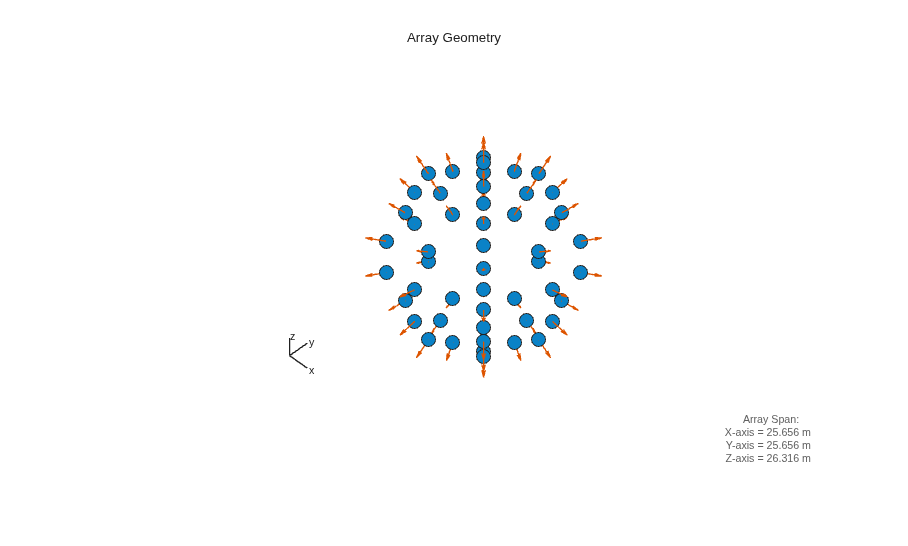
The transmitter consists of a hemispherical array of back-baffled isotropic projector elements. The transmitter is located 60 meters below the surface. Create the array and view the array geometry.
plat = phased.Platform(...
    'InitialPosition',[0; 0; -60],...
    'Velocity',[0; 0; 0]);

proj = phased.IsotropicProjector(...
    'FrequencyRange',[0 30e3],'VoltageResponse',80,'BackBaffled',true);

[ElementPosition,ElementNormal] = helperSphericalProjector(8,fc,propSpeed);

projArray = phased.ConformalArray(...
    'ElementPosition',ElementPosition,...
    'ElementNormal',ElementNormal,'Element',proj);

viewArray(projArray,'ShowNormals',true);
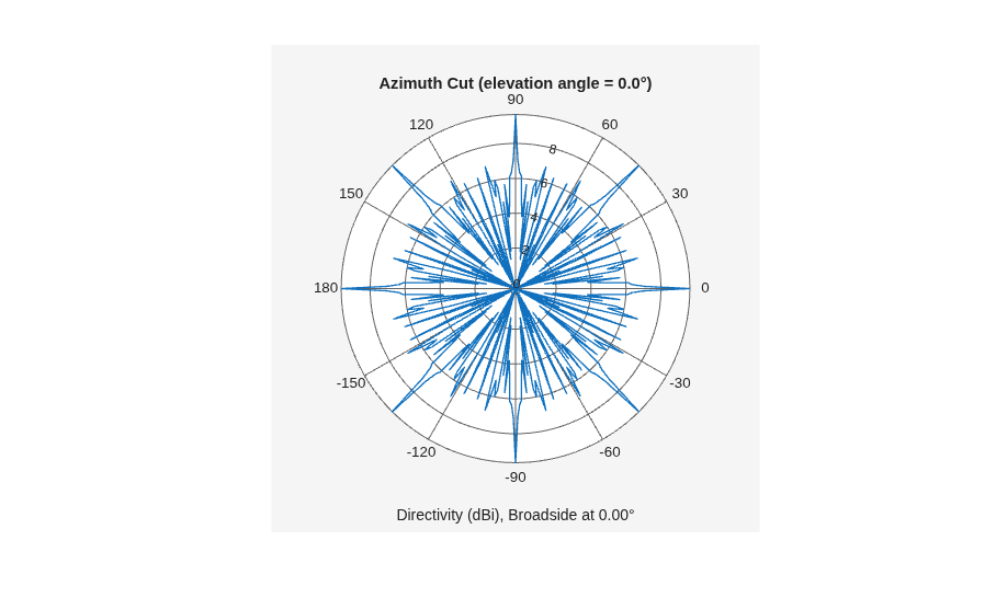
View the pattern of the array at zero degrees in elevation. The directivity shows peaks in azimuth corresponding to the azimuth position of the array elements.
pattern(projArray,fc,-180:180,0,'CoordinateSystem','polar',...
      'PropagationSpeed',propSpeed);
Receiver
The receiver consists of a hydrophone and an amplifier. The hydrophone is a single isotropic element and has a frequency range from 0 to 30 kHz, which contains the operating frequency of the multipath channel. Specify the hydrophone voltage sensitivity as -140 dB.
hydro = phased.IsotropicHydrophone(...
    'FrequencyRange',[0 30e3],'VoltageSensitivity',-140);
Thermal noise is present in the received signal. Assume that the receiver has 20 dB of gain and a noise figure of 10 dB.
rx = phased.ReceiverPreamp(...
    'Gain',20,...
    'NoiseFigure',10,...
    'SampleRate',fs,...
    'SeedSource','Property',...
    'Seed',2007);
Radiator and Collector
In an active sonar system, an acoustic wave is propagated to the target, scattered by the target, and received by a hydrophone. The radiator generates the spatial dependence of the propagated wave due to the array geometry. Likewise, the collector combines the backscattered signals received by the hydrophone element from the far-field target.
radiator = phased.Radiator('Sensor',projArray,'OperatingFrequency',...
 fc,'PropagationSpeed',propSpeed);

collector = phased.Collector('Sensor',hydro,'OperatingFrequency',fc,...
  'PropagationSpeed',propSpeed);
Sonar System Simulation
Next, transmit the rectangular waveform over ten repetition intervals and simulate the signal received at the hydrophone for each transmission.
x = wav();    % Generate pulse
xmits = 10;
rx_pulses = zeros(size(x,1),xmits);
t = (0:size(x,1)-1)/fs;

for j = 1:xmits

    % Update target and sonar position
    [sonar_pos,sonar_vel] = plat(1/prf);

    for i = 1:2 %Loop over targets
       [tgt_pos,tgt_vel] = tgtplat{i}(1/prf);

      % Compute transmission paths using the method of images. Paths are
      % updated according to the CoherenceTime property.
      [paths,dop,aloss,tgtAng,srcAng] = isopath{i}(...
            sonar_pos,tgt_pos,...
            sonar_vel,tgt_vel,1/prf);

      % Compute the radiated signals. Steer the array towards the target.
      tsig = radiator(x,srcAng);

      % Propagate radiated signals through the channel.
      tsig = channel{i}(tsig,paths,dop,aloss);

      % Target
      tsig = tgt{i}(tsig,tgtAng);

      % Collector
      rsig = collector(tsig,srcAng);
      rx_pulses(:,j) = rx_pulses(:,j) + ...
               rx(rsig);
    end
end
Plot the magnitude of non-coherent integration of the received signals to locate the returns of the two targets.
figure
rx_pulses = pulsint(rx_pulses,'noncoherent');
plot(t,abs(rx_pulses))
grid on
xlabel('Time (s)')
ylabel('Amplitude (V)')
title('Integrated Received Pulses')
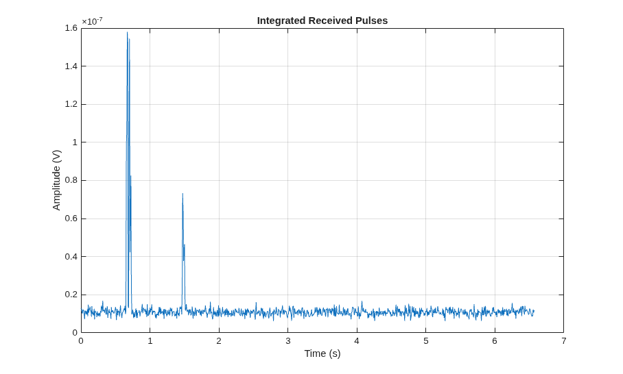
The targets, which are separated a relatively large distance, appear as distinct returns. Zoom in on the first return.
xlim([0.55 0.85])
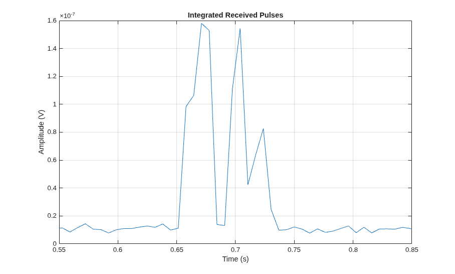
The target return is the superposition of pulses from multiple propagation paths, resulting in multiple peaks for each target. The resulting peaks could be misinterpreted as additional targets.
Summary
In this example, acoustic pulses were transmitted and received in a shallow-water environment. Using a rectangular waveform, an active sonar system detected two well-separated targets in shallow water. The presence of multiple paths was apparent in the received signal.
The Deep Underwater Channel Target Detection Using Active Sonar example uses Bellhop beam tracing model to simulate target detection using active sonar in a deep-channel environment.
Reference
Urick, Robert. Principles of Underwater Sound. Los Altos, California: Peninsula Publishing, 1983.

