Using NPoles Parameter with rationalfit
This example shows how to use the NPoles parameter to improve the quality of the output of rationalfit. By default, the rationalfit function uses 48 or fewer poles to find the rational function that best matches the data. If 48 poles is not enough, it may be advantageous to change the range of the number of poles used by rationalfit.
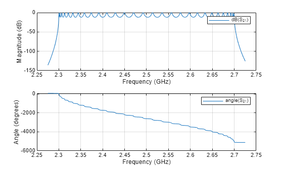
First, read in the bandpass filter data contained in the file npoles_bandpass_example.s2p, and plot the S21 data. Next, use the rationalfit function to fit a rational function to the S21 data, with the NPoles parameter set to its default value, and visually compare the results to the original data. Lastly, use rationalfit again, this time specifying a larger number of poles, and see if the result improves.
Read and Visualize Data
S = sparameters('npoles_bandpass_example.s2p');
figure
subplot(2,1,1)
rfplot(S,2,1,'db')
subplot(2,1,2)
rfplot(S,2,1,'angle')

Analyze Output of rationalfit When Using Default Value for NPoles
Use the rfparam function to extract the S21 values, and then call rationalfit.
s21 = rfparam(S,2,1);
datafreq = S.Frequencies;
defaultfit = rationalfit(datafreq,s21);
Warning: Achieved only -13.0 dB accuracy with 48 poles, not -40.0 dB. Consider specifying a larger number of poles using the 'NPoles' parameter.
Use the freqresp function to calculate the response of the output of rationalfit.
respfreq = 2.25e9:2e5:2.75e9;
defaultresp = freqresp(defaultfit,respfreq);
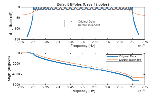
Compare the original data against the frequency response of the default rational function calculated by rationalfit.
subplot(2,1,1)
plot(datafreq,20*log10(abs(s21)),'.-')
hold on
plot(respfreq,20*log10(abs(defaultresp)))
hold off
xlabel("Frequency (Hz)")
ylabel("Magnitude (dB)")
defaultnpoles = numel(defaultfit.A);
defaultstr = ["Default NPoles (Uses ",num2str(defaultnpoles)," poles)"];
title(defaultstr)
legend("Original Data","Default rationalfit",Location="best")
subplot(2,1,2)
plot(datafreq,unwrap(angle(s21))*180/pi,'.-')
hold on
plot(respfreq,unwrap(angle(defaultresp))*180/pi)
hold off
xlabel("Frequency (Hz)")
ylabel("Angle (degrees)")
legend("Original Data","Default rationalfit",Location="best")

Analyzing how well the output of rationalfit matches the original data, it appears that while the default values of rationalfit do a reasonably good job in the center of the bandpass region, the fit is poor on the edges of the bandpass region. It is possible that using a more complex rational function will achieve a better fit.
Analyze Output of rationalfit When Using Custom Value for NPoles
Fit the original S21 data, but this time, instruct rationalfit to use between 49 and 60 poles using the NPoles parameter.
customfit = rationalfit(datafreq,s21,NPoles=[49 60]);
customresp = freqresp(customfit,respfreq);
Compare the original data against the frequency response of the custom rational function calculated by rationalfit.
figure
subplot(2,1,1)
plot(datafreq,20*log10(abs(s21)),'.-')
hold on
plot(respfreq,20*log10(abs(customresp)))
hold off
xlabel("Frequency (Hz)")
ylabel("Magnitude (dB)")
customnpoles = numel(customfit.A);
customstr = ["NPoles = [49 60] (Uses ",num2str(customnpoles)," poles)"];
title(customstr)
legend("Original Data","Custom rationalfit",Location="best")
subplot(2,1,2)
plot(datafreq,unwrap(angle(s21))*180/pi,'.-')
hold on
plot(respfreq,unwrap(angle(customresp))*180/pi)
hold off
xlabel("Frequency (Hz)")
ylabel("Angle (degrees)")
legend("Original Data","Custom rationalfit",Location="best")
![Figure contains 2 axes objects. Axes object 1 with title NPoles = [49 60] (Uses 58 poles), xlabel Frequency (Hz), ylabel Magnitude (dB) contains 2 objects of type line. These objects represent Original Data, Custom rationalfit. Axes object 2 with xlabel Frequency (Hz), ylabel Angle (degrees) contains 2 objects of type line. These objects represent Original Data, Custom rationalfit.](../../examples/rf/win64/UsingTheNpolesParameterWithRationalfitExample_03.png)
The fit using a larger number of poles is clearly more precise.