Filter Designer
Design filters by choosing algorithm or specifying constraints
Description
The Filter Designer app enables you to design and compare digital filters. You can also import existing filter designs from the MATLAB® workspace or from a previously saved app session.
Design and analyze IIR, FIR, and multirate filters by:
Starting with a list of specifications and then choosing the design algorithm that best satisfies them
Starting with your preferred algorithm and then adjusting the algorithm parameters
Adding, removing, or modifying transfer-function poles and zeros.
View each filter response in several ways using different analysis and display options.
After you finish designing a filter, you can:
Export your design to the MATLAB workspace or to Simulink®.
Export filters to DSP HDL IP Designer (DSP HDL Toolbox) if you have a DSP HDL Toolbox™ license.
Generate MATLAB code to recreate your design or filter a signal.
Generate a C header or COE file using coefficients.
If you have a DSP System Toolbox™ license, you can export a design as a filter System object™ or generate MATLAB code to filter a signal using a filter System object.
For more information, see Use Filter Designer App.

Open the Filter Designer App
MATLAB Toolstrip: On the Apps tab, under Signal Processing and Audio, click the app icon.
MATLAB command prompt: Enter
filterDesigner.
Examples
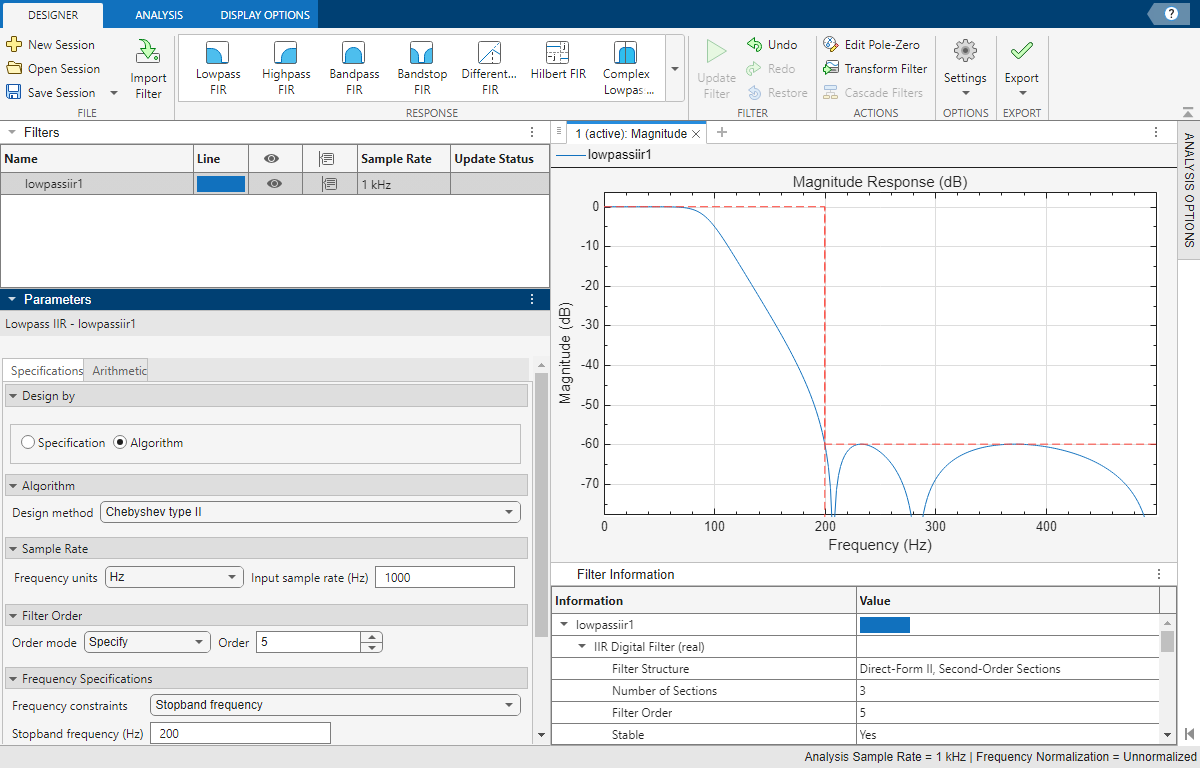
Use the Filter Designer app to create a lowpass filter to preserve frequency content under 200 Hz for signals sampled at 1 kHz. Select the Chebyshev type II algorithm to design a low-order filter with a narrow transition region and no ripple in the passband.
Open Filter Designer.
In the Response gallery of the Designer tab in the app toolstrip, select
Lowpass IIR. The app displays a filter design with default specifications.Under Algorithm, select
Chebyshev type II.Under Sample Rate, select
Hzfor the frequency units and specify the input sample rate as 1000.Under Filter Order, select
Specifyand specify the order as5.Under Frequency Specifications, specify a stopband frequency of
200Hz.In the Filter section of the Designer toolstrip tab, click Update Filter.
Use the Filter Designer app to create a 50th-order FIR bandpass filter to be used with signals sampled at 1 kHz. The desired passband spans frequencies of 200–300 Hz and has a transition region of width 50 Hz on either side. Specify that frequencies in the lower stopband are attenuated by at least 40 dB and frequencies in the upper stopband are attenuated by at least 60 dB.
Open Filter Designer.
In the Response gallery of the Designer tab in the app toolstrip, select
Bandpass FIR. The app displays a filter design with default specifications.Under Sample Rate, set the frequency units to
Hzand specify the sample rate as1000Hz.Under Filter Order, select
Specifyand specify the order as50.Under Frequency Specifications, set the frequency constraints to
Passband and stopband frequencies, and enter these frequency values:150Hz for Stopband frequency 1 (Hz)200Hz for Passband frequency 1 (Hz)300Hz for Passband frequency 2 (Hz)350Hz for Stopband frequency 2 (Hz)
Set the Algorithm to
Equiripple. Under Algorithm Options, set these weight values:3for Stopband weight 11for Passband weight100for Stopband weight 2
In the Filter section of the Designer toolstrip tab, click Update Filter.

Export the code to create your digital filter. On the toolstrip, click
Export and select Generate MATLAB
function > Digital Filter Object. The code
appears in the
Editor.
function designedFilter = bandpassfir1

% Generated by MATLAB(R) 25.2 and Signal Processing Toolbox 25.2.
% Generated on: 19-Dec-2024 18:11:24

designedFilter = designfilt('bandpassfir', ...
    'FilterOrder',50,'StopbandFrequency1',150, ...
    'PassbandFrequency1',200,'PassbandFrequency2',300, ...
    'StopbandFrequency2',350,'SampleRate',1000, ...
    'StopbandWeight1',3,'StopbandWeight2',100);

end
Create a 100th-order arbitrary-magnitude FIR filter. Input the specifications at the MATLAB command line and import them to the Filter Designer app to finalize the design.
The filter has the following piecewise frequency response:
A sinusoid between 0 and 0.19π rad/sample.
F1 = 0:0.01:0.19;
A1 = 0.5+sin(2*pi*7.5*F1)/4;
A piecewise linear section between 0.2π rad/sample and 0.78π rad/sample.
F2 = [0.2 0.38 0.4 0.55 0.562 0.585 0.6 0.78];
A2 = [0.5 2.3 1 1 -0.2 -0.2 1 1];
A quadratic section between 0.79π rad/sample and the Nyquist frequency.
F3 = 0.79:0.01:1;
A3 = 0.2+18*(1-F3).^2;
Consolidate the frequency and amplitude vectors. Open the Filter Designer app.
FreqVect = [F1 F2 F3];
AmplVect = [A1 A2 A3];

filterDesigner
Use the app to design the filter.
In the Response gallery of the Designer tab in the app toolstrip, select
Arbitrary Response FIR. The app displays a filter design with default specifications.Under Filter Order, select
Specifyand specify the order as100.Under Response, set the number of bands to
1and the response type toAmplitudes. In the table, specifyFreqVectfor the Frequencies andAmplVectfor the Amplitudes.Set the Algorithm to
Frequency sampling.In the Filter section of the Designer toolstrip tab, click Update Filter.
Double-click the Analysis Options button at the right of the app window to anchor the Analysis Options pane. In the Magnitude Options section, select
Zero
                    Phase
for the magnitude mode. Click Apply. If you want to minimize the Analysis Options panel, click the Analysis Options button in the Analysis tab of the app toolstrip.

Use the Filter Designer app to create a 150th-order FIR lowpass filter with stepped attenuation levels in the stopband.
Open Filter Designer.
In the Response gallery of the Designer tab in the app toolstrip, select
Arbitrary Response FIR. The app displays a filter design with default specifications.Under Filter Order, select
Specifyand specify the order as150.Under Response, set the number of bands to
2and the response type toAmplitudes. Enter these values:For band 1, the passband, specify
[0 0.25]for the Frequencies andones(1,2)for the Amplitudes.For band 2, the stopband, specify
[0.3 0.4 0.401 0.5 0.501
                          0.6 0.601 0.7 0.701 0.8 0.801 0.9 0.901 1]
for the Frequencies andzeros(1,14)for the Amplitudes.
Under Algorithm Options, set the weights:
For the passband, specify
10.^([0 0]/20).For the stopband, specify
10.^([5 5 10 10 15 15 20 20 25 25
                          30 30 35 35]/20)
.
In the Filter section of the Designer toolstrip tab, click Update Filter.

Parameters
Main Pane
Filters Table
Select a filter in the Filters table to edit its parameters or see its filter information. Interact with the table to change the visualization of each filter.

Name — Double-click an entry in this column to edit the name of the filter. You can also right-click the filter in the Filters table and select Rename.
Line — Click an entry in this column to edit the color used to display that filter response.
Eye — Click an entry in this column to add the corresponding filter to the current display or to remove it. You can also drag filters from the Filters table onto any display for visualization.
Cursor — Click an entry in this column to show or remove data cursors for the corresponding filter. Hover on an entry in this column to switch between showing one cursor or showing two.
Sample Rate — Shows the sample rate for the corresponding filter.
Update Status — Informs when you have modified parameters for a filter but have not yet updated it.
To duplicate, rename, or delete a filter from the app, right-click in the selected filter and select one of these options:
Duplicate — The app names the duplicated filter using the same name as the original one and appends it with the string
_Copy.Rename — Type the new filter name and press Enter. Alternatively, double-click the filter name, type a new filter name, and press Enter.
Delete — Confirm the deletion in the dialog box that appears.
Parameters
After choosing a filter in the Filters table, you can specify your filter further using parameters from this panel. Available specifications are response dependent and include combinations of these:
Sample Rate is the frequency at which the filter operates.
Filter Order specifies the order of the filter. Some design methods let you specify the order. Others produce the smallest filters that satisfy the specified constraints.
Frequency Specifications correspond to the frequencies at which a filter exhibits a desired behavior.
Magnitude Specifications describe the filter behavior at particular frequency ranges.
Algorithm is the method used to design the filter.
Algorithm Options are parameters specific to a given design method.
This panel section is available only for lowpass, highpass, bandpass, and bandstop filters.
You can choose to specify the characteristics of your filter either by:
Specification— Specify the frequency and magnitude constraints first and then choose an algorithm.Algorithm— Choose a design algorithm first and then adjust its parameters.
Specify the input sample rate of the filter in normalized frequency units or in Hz.
You need a DSP System Toolbox license to use this functionality.
This panel section is available only for multirate single-stage FIR filters.
Specify the FIR filter type to use for the multirate filter design as one of these:
Zero-order hold— Generate a zero-order hold multirate FIR filter by using the Lagrange design method with a polyphase length of 1.Linear interpolation— Generate a linear-interpolation multirate FIR filter by using the Lagrange design method with a polyphase length of 2.Lowpass— Generate a lowpass multirate FIR filter by using the Kaiser design method.
For more information about multirate FIR filters, see designMultirateFIR (DSP System Toolbox).
Design a minimum-order filter or specify a filter order. Some responses might not have a minimum order design available and will require you to specify a filter order value.
In some design cases, there are model order restrictions. If an even or odd restriction exists for the selected design method and the specified order is not valid, Filter Designer increases the order by one.
For more information, see Filter Order.
This panel section is available only for arbitrary-response filters.
Specify the number of bands and the response at which the designed filter exhibits a desired behavior. Available response types are as follows:
Amplitudes— Specify the vector of frequencies and amplitudes that represents the desired filter amplitude response in each band. For a multiband filter, you can also specify the magnitude ripple constraint in each band.Magnitudes and phases— Specify the vector of frequencies, magnitudes, and phases that represent the desired filter response in each band.This option requires a DSP System Toolbox license.
Frequency response— Specify the vector of frequencies and complex-valued responses that represent the desired filter response in each band.This option requires a DSP System Toolbox license.
Note
If you set multiple bands, Filter Designer updates
the design method from Frequency
Sampling to
Equiripple.
This panel section is available only for fractional-delay FIR filters and requires a DSP System Toolbox license.
Specify the fractional delay in samples of the filter. For more
information, see FractionalDelay.
You need a DSP System Toolbox license to use this functionality.
This panel section is available only for Multinotch IIR, Multipeak IIR, Halfband FIR, and Halfband IIR responses.
For multi-notch IIR and multi-peak IIR filters, specify the source of notch frequencies or peak frequencies. When you select:
Specify— Manually set the notch or peak frequencies.The filter order associated with each notch or peak can be a scalar or a vector of size equal to the number of notches or peaks. If you specify the filter order as a scalar, the app assumes that the filter order is the same across all notches or peaks.
Harmonic— Use harmonic frequencies. The notches or peaks are uniformly spaced in the frequency range.
For halfband FIR and IIR filters, set the filter order mode and the response type.
Set the filter order mode as one of these:
Minimum— Design a minimum order filter that meets the design specifications.Specify— Specify the filter order and other design specifications such as the transition width and the stopband attenuation.
If the rate specification under the Sample Rate section is
Single-rate, you can specify the response type asLowpassorHighpass.
Specify the frequencies at which the designed filter exhibits a desired behavior. Available options depend on filter response type and filter order.
For more information, see Frequency Constraints.
Choose the filter magnitude response behavior at the specified frequency ranges. Available options depend on filter response type, filter order, and frequency specifications.
For more information, see Magnitude Constraints.
Specify the algorithm used to design the filter. Available options depend on filter response type, filter order, and frequency and magnitude constraints. Some design methods have additional options available in the Algorithm Options section.
For more information, see Design Method.
Available options depend on the chosen algorithm.
For more information, see Design Method Options.
You need a DSP System Toolbox license and a Fixed-Point Designer™ license to use this functionality.
This panel section is available only for Compensated CIC Filter response.
Specify the CIC filter type as one of these:
Standalone CIC filter— Generate a CIC decimation filter (dsp.CICDecimator(DSP System Toolbox)) or a CIC interpolation filter (dsp.CICInterpolator(DSP System Toolbox)).Compensated CIC filter— Generate adsp.FilterCascade(DSP System Toolbox) object with one of these as stages:dsp.CICDecimator(DSP System Toolbox) anddsp.CICCompensationDecimator(DSP System Toolbox) objectsdsp.CICInterpolator(DSP System Toolbox) anddsp.CICCompensationInterpolator(DSP System Toolbox) objects
CIC filters are always fixed-point.
You need a DSP System Toolbox license and a Fixed-Point Designer license to use this functionality.
This panel section is available only for Compensated CIC Filter response.
Specify the differential delay and the number of sections of the CIC filter. For more information on these two parameters, see one of these object pages depending on the CIC filter type.
dsp.CICDecimator(DSP System Toolbox)dsp.CICCompensationDecimator(DSP System Toolbox)dsp.CICInterpolator(DSP System Toolbox)dsp.CICCompensationInterpolator(DSP System Toolbox)
You can specify the rate conversion factor of the CIC filter and the CIC compensation filter using the settings in the Sample Rate panel.
You need a DSP System Toolbox license and a Fixed-Point Designer license to use this functionality.
This panel section is available only when you set the response and
CIC filter type to Compensated CIC
filter.
Specify the filter order, frequency specifications, and magnitude
specifications of the CIC compensation decimation filter and CIC
compensation interpolation filter. For more information on these
parameters, see dsp.CICCompensationDecimator (DSP System Toolbox)
and dsp.CICCompensationInterpolator (DSP System Toolbox).
After designing your filter, specify the filter arithmetic using the settings in this panel.
Specify the filter arithmetic to use to quantize the filter
coefficients as Double precision,
Single precision, or Fixed
point.
When you set Arithmetic to Fixed
point:
The app quantizes the designed filter based on the fixed-point coefficient settings that you specify in the Coefficient Quantization panel.
The analysis plot shows the frequency response of the reference filter with floating-point coefficients and the quantized filter with fixed-point coefficients.
The Filter Information panel in the app shows the fixed-point arithmetic and filter coefficient information.
Note
To use the fixed-point arithmetic, you must have licenses for DSP System Toolbox and Fixed-Point Designer.
You can export and share the quantized filter to use it in different workflows. For more information, see Quantize Filters (DSP System Toolbox).
This panel tab requires a DSP System Toolbox license.
Implement the designed filter as a multirate filter — interpolator, decimator, or a sample-rate converter.
The settings in this section depend on the filter response you choose and the setting of the Rate specification parameter. When you set the Rate specification parameter to one of these:
Single-rate— The app implements a single-rate filter.Decimator— The app implements a decimator with the decimation factor that you specify.When you specify the input sample rate in Hz, the app displays the conversion ratio, the input sample rate, the filter sample rate, and the output sample rate in this panel.
Interpolator— The app implements an interpolator with the interpolation factor that you specify. You can select whether to scale the passband gain by the interpolation factor.When you specify the input sample rate in Hz, the app displays the conversion ratio, the input sample rate, the filter sample rate, and the output sample rate in this panel.
Sample-rate converter— The app implements the filter as a sample-rate converter with the rate conversion factors that you specify. You can also select whether to scale the passband gain by the interpolation factor.When you specify the input sample rate in Hz, the app displays the conversion ratio, the input sample rate, the filter sample rate, and the output sample rate in this panel.
Filter Information Table
After selecting a filter in the Filters table, you can see its filter information.
Display filter information including design specifications and design options.
If you have a DSP System Toolbox license, Filter Designer also displays filter measurements.
Designer Tab
Create a new app session, open an existing session, or save session to file.
Note
Filter Designer does not support some of the design options available in previous versions. For more information, see New Filter Designer app replaces previous versions and provides similar functionality with new and updated features.
Click New Session to clear all the data from the current session and start a new session.
Click Open Session to open a Filter Design session file. The app accepts session files created with previous versions.
Click Save Session or Save Session As to save the state of the current session—including filters, displays, and analysis options—as a MAT file for use in a future session of the app.
Click Import Filter to import filter designs that you can visualize and modify using Filter Designer.
Note
If you want to modify an imported filter design using Filter Designer, your design must contain design metadata. Filter designs include design metadata when generated using
designfilt, the Design Filter Live Editor task, System object design functions, or the Filter Designer app itself.Filter Designer does not support
dfiltobjects. If you have filter designs specified asdfiltobjects, you can extract the coefficients from the objects. Alternatively, if you have a DSP System Toolbox license you can use thesysobjfunction to convert adfiltobject to a System object.You cannot modify designs specified as coefficients, but you can use them as reference to compare to new designs. You can also export these designs back to the MATLAB workspace or use them to create Simulink models consisting of atomic elements like delays, adders, and multipliers.
Filter Designer supports these filter types:
digitalFilterObjects — You can use Filter Designer to design and modifydigitalFilterobjects. To generate or edit digital filters based on frequency-response specifications at the command line, usedesignfilt.Filter System objects — If you have DSP System Toolbox, then Filter Designer supports filter System objects. For more information, see Supported Filter System Objects (DSP System Toolbox).
If you select a filter System object, specify the Arithmetic option to set the coefficient quantization arithmetic of the filter as double-precision, single-precision, or fixed-point.
Note
To use fixed-point arithmetic, you must have a DSP System Toolbox license and a Fixed-Point Designer license.
Filter coefficients — You can use Filter Designer to import and display filter coefficients specified in cascaded transfer functions (CTF) format. In particular, you can import designs expressed as numerator and denominator coefficients. For more information, see Import and Export Filter Coefficients.
Example: d = digitalFilter([2 4 2;3 2 0],[1 0 0;1 1 0],[1.4;1.4;5]) specifies a digitalFilter object.
Example: sysObj = dsp.HighpassFilter(FilterType="iir",PassbandRipple=0.2) specifies a DSP System object.
Example: [B,A] = zp2ctf([-1 -1 -1 -1], [0.2i -0.2i 0.66i -0.66i],9) and g=[1.4 1.4 5]' specify a digital filter with CTF numerator and denominator coefficients B and A, respectively. The scalar g represents the scaling gain of the filter.
Choose a filter response to create a filter design of that type.
Tip
To see and access the parameters available for each response type, use the Parameters panel on the main pane of the app. If you have a DSP System Toolbox license, Filter Designer supports additional design specifications in each response.
FIR Specifications
| Response | Icon | Description |
|---|---|---|
| Lowpass FIR | Lowpass FIR filter | |
| Highpass FIR | Highpass FIR filter | |
| Bandpass FIR | Bandpass FIR filter | |
| Bandstop FIR | Bandstop FIR filter | |
| Differentiator FIR | Differentiator FIR filter | |
| Hilbert FIR | Hilbert FIR filter | |
| Complex Lowpass FIR | Complex lowpass FIR filter | |
| Complex Highpass FIR | Complex highpass FIR filter | |
| Arbitrary Response FIR | Arbitrary response FIR filter |
If you have a DSP System Toolbox license, Filter Designer supports these additional responses.
| Response | Icon | Description |
|---|---|---|
| Inverse Sinc Lowpass FIR | Inverse sinc lowpass FIR filter | |
| Inverse Sinc Highpass FIR | Inverse sinc highpass FIR filter | |
| Fractional Delay FIR | Fractional-delay FIR filter |
IIR Specifications
| Response | Icon | Description |
|---|---|---|
| Lowpass IIR | Lowpass IIR filter | |
| Highpass IIR | Highpass IIR filter | |
| Bandpass IIR | Bandpass IIR filter | |
| Bandstop IIR | Bandstop IIR filter |
If you have a DSP System Toolbox license, Filter Designer supports these additional responses.
| Response | Icon | Description |
|---|---|---|
| Arbitrary Response IIR | Arbitrary response IIR filter | |
| Arbitrary Group Delay IIR | Arbitrary group delay IIR filter | |
| Multinotch IIR | Multinotch IIR filter | |
| Multipeak IIR | Multipeak IIR filter |
Multirate Specifications
Note
These responses are available only if you have a DSP System Toolbox license.
For the Compensated CIC Filter response, you must also have a Fixed-Point Designer license.
| Response | Icon | Description |
|---|---|---|
| Sample Rate Converter | Multistage sample-rate converter filter | |
| Multirate Single-Stage FIR | Single-stage polyphase FIR multirate filter | |
| Compensated CIC Filter | Compensated cascaded integrator-comb (CIC) multirate filter | |
| Halfband FIR | Halfband FIR filter | |
| Halfband IIR | Halfband IIR filter |
The buttons in this section enable you to commit or undo any changes you make to a filter design.
Click Update filter to design the selected filters using the current parameters.
Click Undo to undo the last update you made to the selected filter.
Click Redo to redo the last update you made to the selected filter.
Note
To commit any changes that you make to a filter design, click the Update Filter button.
The buttons in this section enable you to edit poles and zeros, apply filter transformations, and produce more elaborate filters by cascading simpler filters.
Click Edit Pole-Zero to enter the Edit Pole-Zero Tab mode and edit the poles and zeros of the selected filter.
Note
Pole-zero editing is not supported for digital filter cascades.
This option requires a DSP System Toolbox license.
Click Transform Filter to flip, invert, or transform the selected FIR or IIR filter into another form to achieve a target frequency response.
Note
Multirate filters and digital filter cascades do not support frequency transformation.
In the dialog box that appears, set these options:
Transform Type — Flip, invert, or frequency-transformation algorithm used to convert a lowpass filter prototype into a target filter with a different response. The available algorithms depend on the response of the filter you select for transformation.
If you select a real FIR or IIR filter, the app lists only real frequency transformations. For more information, see Frequency Transformations for Real Filters (DSP System Toolbox).
If you select a complex FIR filter, the app lists only complex frequency transformations. For more information, see Frequency Transformations for Complex Filters (DSP System Toolbox).
Frequency Units — Frequency units to use for the filter transformation, specified as
Normalized(rad/sample) or units of cyclical frequencies (Hz,kHz,MHz, orGHz).Original Frequency — Frequency of the lowpass filter prototype used for the filter frequency transformation.
Target Frequency — Frequency of the target filter resulting from the filter frequency transformation.
Overwrite Filter — Select this option to overwrite the original filter with the transformed filter. If you do not select this option, Filter Designer creates the transformed filter as a new filter.
Click Cascade Filters to create a cascade filter using the selected filters.
Note
All the filters selected for cascading must use the same coefficient quantization arithmetic.
In the dialog box that appears, set up the filter cascade:
Stages — The top and bottom rows list the first and last stages of the digital filter cascade, respectively. To sort the filter stages, drag a filter row-wise or select the filter and use the Move Up and Move Down buttons.
Frequency Units — Specify Frequency Units as one of these:
Auto— Filter Designer automatically sets the sample rate of the filter cascade. All the selected filters must use the same sample rate or use normalized frequency.Normalized— Filter Designer sets all the stages to use normalized frequency in radians per sample.Specify— Specify the sample rate of the filter cascade and its corresponding unit.
Sample Rate — Set Sample Rate with the sample rate of the filter cascade and its corresponding unit.
To choose to overwrite variables of the same name when you export filters to the MATLAB workspace, click Settings and select the check box.
Use the Export button to export filter designs to the MATLAB workspace or Simulink and generate MATLAB code to implement your filter designs or use them to process signals.
To export a design, select a filter in the Filters table and use one of these options:
Click an option to generate variables in the MATLAB workspace from a selected filter.
Digital Filter Object— Create adigitalFilterobject that represents the selected filter.Filter System Object— Create a filter System object that represents the selected filter. The filter System object that Filter Designer creates depends on the filter selected for export.This option requires a DSP System Toolbox license.
Coefficients— Create a set of one or two matrices that represents the numerator and denominator coefficients of the selected filter. Filter Designer exports the coefficients as matrices of cascaded second-order transfer functions, each with unit gain.
Note
Multirate filters do not support export as digital filter objects.
Compensated CIC, and halfband IIR filters do not support export as coefficients.
Multipeak IIR filters do not support export as digital filter objects or coefficients, unless the filter has only one peak.
Click an option to create a Simulink block from a selected filter. You must have Simulink installed to create Simulink blocks.
DSP filter block— Implement the selected filter as a DSP filter block. The filter block that Filter Designer creates depends on the filter selected for export.This option requires a DSP System Toolbox license.
System of basic elements— Implement the selected filter in Simulink as a Subsystem (Simulink) block that uses basic blocks, including Sum (Simulink), Gain (Simulink), and Delay (Simulink).
Note
You must have DSP System Toolbox and Fixed-Point Designer installed to export a compensated CIC filter to Simulink.
In the dialog box that appears once you choose the export type, set up the export.
Overwrite filter block — Select this option to overwrite a previously generated DSP filter block or system of basic elements.
Model — Select the target Simulink model where the app adds the exported DSP filter block or system of basic elements.
Opened (current)— Use the open Simulink model that you most recently interacted with. If no model is open in Simulink, then the app opens a new one.New— Use a new Simulink model.Opened (other)— Use an open Simulink model with a name that you specify. When you type the model name, do not include the.slxextension.
Filter Structure (for export to system of basic elements only) — Select one of the filter structures available to implement the filter in Simulink, depending on the filter selected for export.
Selected Filter Filter Structures FIR Direct-form FIR, direct-form transposed FIR, direct-form symmetric FIR, direct-form antisymmetric FIR, or overlap-add FIR
For more information, see Discrete FIR Filter (Simulink).IIR Direct-form I SOS, direct-form II SOS, direct-form I transposed SOS, or direct-form II transposed SOS
For more information, see Second-Order Section Filter (DSP System Toolbox).Halfband FIR Direct-form FIR polyphase decimator, direct-form transposed FIR polyphase decimator
For more information, see FIR Halfband Decimator (DSP System Toolbox).Halfband IIR IIR polyphase decimator, IIR wave digital filter polyphase decimator
For more information, see IIR Halfband Decimator (DSP System Toolbox).Optimization (for export to system of basic elements only) — Select the optimizations available to simplify the Simulink model.
Zero gains— Removes zero-valued gain paths from the filter structure.Unity gains— Substitutes a wire (short circuit) for gains equal to 1 in the filter structure.Negative gains— Substitutes a wire (short circuit) for gains equal to -1 and changes corresponding additions to subtractions in the filter structure.Delay chains— Substitutes delay chains composed of n unit delays with a single delay of n.Unity scale values—Removes multiplications for scale values equal to 1 from the filter structure.
Input Processing — Select whether the Simulink block uses framed-based or sample-based processing algorithms for input signals. Depending on the type of filter you design, one or both of these options are available:
Columns as channels (frame
                                                  based)
— The block treats each column of the input as a separate channel.Elements as channels (sample based)— The block treats each element of the input as a separate channel.
For more information, see Sample- and Frame-Based Concepts (DSP System Toolbox).
Rate Options (for certain multirate filters only) — Depending on the selected filter and the export type, Filter Designer selects a rate option for the exported block, either as
Enforce single rate processingorAllow multirate processing.
This option requires a DSP HDL Toolbox license.
Click this option to open a session in the DSP HDL IP Designer (DSP HDL Toolbox) app and load the selected filter on the session. In the DSP HDL IP Designer session, you can configure the app and generate HDL code. To learn more, see Generate and Verify HDL Code with DSP HDL IP Designer App (DSP HDL Toolbox).
Note
Digital filter cascades do not support export to DSP HDL IP Designer.
Click an option to generate a MATLAB function from a selected filter.
Digital Filter Object— Generate a MATLAB function that returns adigitalFilterobject representing the selected filter.Filter System Object— Generate a MATLAB function that returns a System object representing the selected filter.This option requires a DSP System Toolbox license.
Filtering with System Object— Generate a MATLAB function that filters a signal using a System object representing the selected filter. The generated MATLAB function declares the input signal as an input argument.This option requires a DSP System Toolbox license.
Note
Multirate filters do not support export as digital filter objects.
Multipeak IIR filters do not support export as digital filter objects, unless the filter has only one peak.
Click an option to export the coefficients of a selected filter to a file.
Generate C Header— Create a C header (.h) file that contains the coefficients of the selected filter. You can include C header files in external C programs. In the dialog box that appears, specify the variable names for the filter coefficients and filter coefficient length, and the filter data type.Generate COE File— Create a Xilinx® coefficients (.coe) file that contains the coefficients of the selected quantized filter.This option requires a DSP System Toolbox and Fixed-Point Designer license.
Note
Variable names cannot be C language reserved words, such as “for” or “if”.
If you do not have DSP System Toolbox installed, selecting any data type other than double-precision floating point might produce a filter that differs from the one designed in Filter Designer due to coefficient rounding and truncation in the filter coefficients.
Multipeak IIR filters and multirate filters do not support C-header file generation.
Complex FIR, IIR and multirate filters do not support COE file generation.
Analysis Tab
Click Duplicate Display to duplicate the active display.
Click New Display to add a new blank display.
Click Copy Display to copy the active display to the clipboard.
Tip
You can alternatively right-click the plotting area on the active display and select Copy Display to Clipboard.
Expand this gallery to choose a base and optional secondary analysis for the active display. Choose options using the thumbnail view or the details view of the gallery.
Analysis — Choose the base analysis type.
Overlay Analysis — Optionally, choose the secondary analysis that overlays the base analysis.
To access the options available for each analysis, use the Analysis Options button in the Analysis Options toolstrip section.
Filter Designer supports the analysis types listed in the table.
Frequency-Domain Analyses
| Analysis | Icon | Options | Description |
|---|---|---|---|
| Magnitude response | Magnitude Mode: Select Normalize Magnitude: Toggle on or off |
Tip If you select this analysis, you can zoom in the response to the passband or stopband. Hover on the top-right corner of the display and click the or icons. | |
| Phase response | Phase Units: Select Phase Display: Select | ||
| Group delay response | Group Delay Units: Select Samples or Time |
| |
| Phase delay response | Phase Units: Select Radians or Degrees |
|
Time-Domain Analyses
| Analysis | Icon | Options | Description |
|---|---|---|---|
| Impulse response | Specify Length: Select Auto or User-defined |
| |
| Step response | Specify Length: Select Auto or User-defined |
|
Other Analyses
| Analysis | Icon | Options | Description |
|---|---|---|---|
| Pole-zero plot | N/A |
| |
| Filter coefficients | Coefficients Format: Select Decimal, Hexadecimal, or Binary |
| |
| Filter information | N/A |
|
Frequency Normalization
In Filter Designer, you can display filter responses using normalized frequencies or in terms of a sample rate of your choice. To select how to display frequencies, in the Analysis Options section of the Analyzer tab, set Frequency Normalization to one of these values.
Auto— If some filters do not have a sample rate, the app analyzes filter responses using normalized frequencies measured in rad/sample. If all filters have a sample rate, the app analyzes filter responses using cyclical frequencies measured in Hz.Normalized— The app analyzes filter responses using normalized frequencies measured in rad/sample.Unnormalized— The app analyzes filter responses using cyclical frequencies measured in Hz.
Analysis Sample Rate
You can choose a reference sample rate, to use to compare the filters plotted in a display to each other, by entering a value for Analysis Sample Rate. You can also choose the highest sample rate among all the filters in the display by selecting Max. To edit the sample rate units, click the pencil icon.
Analysis Options
Select Analysis Options to open the Analysis Options pane, which contains these options for all frequency-domain analyses:
Frequency Scale — To display responses in linear frequency scale, select
Linear. To use a logarithmic frequency scale, selectLog.Frequency Range — To display responses over positive frequencies only, select
One Sided. To display responses over the whole frequency range, selectTwo Sided. To display responses over the whole frequency range centered at zero, selectCentered. To display responses over a custom range of frequencies, selectUser-defined.By default, the app displays one-sided responses if all filters under analysis in a display have real-valued coefficients and centered responses if at least one filter has complex-valued coefficients.
Number of Points — Select the number of discrete Fourier transform points you want to use to display frequency-domain responses.
For a list of options available with each analysis type, see Analysis.
Click Default Layout to restore the display layout. When you click this button, Filter Designer arranges all displays into a single tile, while preserving the analysis plots and options within in each display.
Display Options Tab
Filter Designer supports these display options:
Legend — Toggle to show or hide legends in the active display. To show or hide the legend in all displays, click Legend▼ and select
Show All LegendsorHide All Legends, respectively.Grid — Toggle to show or hide the grid in the active display. To show or hide the grid in all displays, click Grid▼ and select
Show All GridsorHide All Grids, respectively.Hide Cursors — Click to hide the cursors in the active display. To hide the data cursors in all displays, click Hide Cursors▼ and select
Hide All Cursors.To show the cursor corresponding to a given filter, click the cursor column of a signal in the Filters table.
Click Mask to show or hide the spectral mask in the active display. You can use a standard filter specification mask or you can define your own.
In Filter Designer, a mask is a plot that outlines the passband ripples, stopband attenuation, and transition width of the filter. Showing a mask in the magnitude response serves as a visual reference that aids you to compare the expected magnitude and frequency specifications with the actual filter response, which can help you assess the filter design.
If the filter being plotted in the active display has design specifications, then the app can draw a specifications-based mask.
Note
To use standard specification masks, filters must have design metadata. To include metadata in your design, use a
digitalFilterobject or a filter System object.If you define your own mask, then the app can draw a user-defined mask, based on the mask frequencies and magnitudes that you specify.
Specify a custom mask as a set of frequencies and a corresponding set of values. To specify your selection, click User Settings. You can use normalized frequencies or express frequencies in units of Hz, kHz, MHz, or GHz. You can specify values for the magnitude of interest, the square of the magnitude, or the magnitude expressed in dB. The frequencies and the values must be finite.
For IIR designs that result in filters with second-order cascaded sections, or for filters imported as cascaded transfer functions, you can choose the way that Filter Designer displays section-by-section responses. This option applies only for displays with one filter. In the Display Options toolstrip tab, click CTF View to toggle between displaying the overall response and displaying the responses section by section. Click CTF View ▼ to select one of these options:
Individual — Show filter responses of individual sections.
Cumulative — Show filter responses of cumulative sections.
User-defined — Show filter responses of selected sections or combinations of sections. To specify your selection, click User Settings and specify Sections a cell array.
For example, assume a CTF of sections numbered from 1 through 7:
{1:7}or{[1 2 3 4 5 6 7]}directs the app to display the response for the entire CTF at once.{1 2 6 7}directs the app to display responses for the CTF section 1, CTF section 2, CTF section 6, and CTF section 7.{[1 2 3] [4 5 7]}directs the app to display responses for a first CTF that comprises the sections 1, 2, and 3, and a second CTF that comprises the sections 4, 5, and 7.{1 [2:4] [6 7]}directs the app to display responses for CTF section 1, the CTF of sections 2 through 4, and the CTF of sections 6 and 7.
Click Reference Filters to show or hide double-precision reference responses for quantized filters in the active display.
When you enable Reference Filters, the app:
Displays the responses of all the selected filters using solid lines
Displays the reference responses using dotted lines
Appends the string
QuantizedorReferenceto each legend entry
Click Polyphase View to show or hide polyphase
decompositions of polyphase filters in the active display. For more
information about polyphase decomposition of multirate filters, see
polyphase (DSP System Toolbox).
When you enable Polyphase View, the app
displays the response for each decomposed phase of the filters you
select for visualization. If a filter has multiple polyphase sections,
then Filter Designer appends the string Polyphase
( to each legend entry,
where p)p varies from 1 to the number of
polyphase sections.
Edit Pole-Zero Tab
Note
This tab appears when you select Edit Pole-Zero on the Designer toolstrip tab.
The Filter field and the Section drop-down list the digital filter and CTF section (for some IIR filters) to whose poles and zeros are being edited.
If the filter has multiple CTF sections, Filter Designer shows the poles and zeros of the first section by default. To select a different filter section, choose a section number from the Section drop-down list.
To select or add a pole or zero, click any of these:
Select — Select a pole or zero in the z-plane.
Add Pole — Add a pole at the selected location in the z-plane.
Add Zero — Add a zero at the selected location in the z-plane.
If Pair is enabled, you can then select or add a conjugate pair of poles or zeros. For more information, see Options.
Set these options to apply a gain to the magnitude response of the filter or to select conjugate pairs.
Gain — Specify a real-valued factor to compensate for the filter's pole(s) and zero(s) gains. This option does not affect the pole or zero, but offsets the magnitude response of the filter when plotted in decibels.
Pair — Enable this option to select or add a pair of conjugate poles or zeros.
When you select a pole or zero from a conjugate pair and if Pair is enabled, then Filter Designer selects both poles or zeros from the conjugate pair.
When you click Add Pole or Add Zero and if Pair is enabled, then Filter Designer adds a conjugate pair of poles or zeros.
Once you select a pole, a zero, or a pair of either, you can drag them to a new location in the z-plane. In this toolstrip tab section, you can perform these operations:
Coordinates — Choose between rectangular and polar coordinates to set the location of a pole or zero.
Polar(default) — Set the Magnitude and Angle (radians) components to the selected pole or zero.Rectangular— Set the Real and Imaginary components to the selected pole or zero.
Flip — Move the selected poles and zeros to their mirrored position.
Flip Along Horizontal Axes — Switch the sign of the imaginary coordinate component.
Flip Along Vertical Axes — Switch the sign of the real coordinate component.
Flip Along Unit Circle — Switch the magnitude |z| to its reciprocal value 1/|z|.
Mirror — Copy the selected poles and zeros and paste them on their mirrored position.
Mirror Along Horizontal Axes — Switch the sign of the imaginary coordinate component.
Mirror Along Vertical Axes — Switch the sign of the real coordinate component.
Mirror Along Unit Circle — Switch the magnitude |z| to its reciprocal value 1/|z|.
Delete — Delete the selected poles and zeros from the filter transfer function.
Rotation (radians) — Set a positive or a negative angle to make a counterclockwise or clockwise rotation to the selected poles or zeros from the z-plane origin, respectively. After rotating, this value reverts to 0.
Scaling factor — Set a real-valued scaling factor to multiply the magnitude of the selected poles or zeros. After scaling, this value reverts to 1.
To exit the pole-zero editor, click one of these:
Accept All — Apply all the pole-zero edits and close the editor. In the dialog box that appears, confirm whether to overwrite the existing filter or create a new one with the applied pole-zero edits.
Cancel — Undo all the pole-zero edits and close the editor.