stft
Short-time Fourier transform
Syntax
Description
s = stft(x)x.
s = stft(___,Name=Value)
stft(___) with no output arguments plots the
magnitude squared of the STFT in decibels in the current figure window.
Examples
Generate a chirp with sinusoidally varying frequency. The signal is sampled at 10 kHz for two seconds.
fs = 10e3;
t = 0:1/fs:2;
x = vco(sin(2*pi*t),[0.1 0.4]*fs,fs);
Compute the short-time Fourier transform of the chirp. Divide the signal into 256-sample segments and window each segment using a Kaiser window with shape parameter β = 5. Specify 220 samples of overlap between adjoining segments and a DFT length of 512. Output the frequency and time values at which the STFT is computed.
[s,f,t] = stft(x,fs,Window=kaiser(256,5),OverlapLength=220,FFTLength=512);
The magnitude squared of the STFT is also known as the spectrogram. Plot the spectrogram in decibels. Specify a colormap that spans 60 dB and whose last color corresponds to the maximum value of the spectrogram.
sdb = mag2db(abs(s));
mesh(t,f/1000,sdb);

cc = max(sdb(:))+[-60 0];
ax = gca;
ax.CLim = cc;
view(2)
colorbar
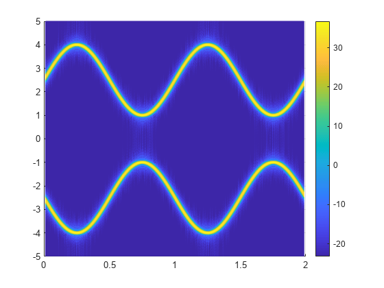
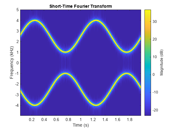
Obtain the same plot by calling the stft function with no output arguments.
stft(x,fs,Window=kaiser(256,5),OverlapLength=220,FFTLength=512)
Generate a quadratic chirp sampled at 1 kHz for 2 seconds. The instantaneous frequency is 100 Hz at and crosses 200 Hz at second.
ts = 0:1/1e3:2;

f0 = 100;
f1 = 200;

x = chirp(ts,f0,1,f1,"quadratic",[],"concave");
Compute and display the STFT of the quadratic chirp with a duration of 1 ms.
d = seconds(1e-3);
win = hamming(100,"periodic");

stft(x,d,Window=win,OverlapLength=98,FFTLength=128);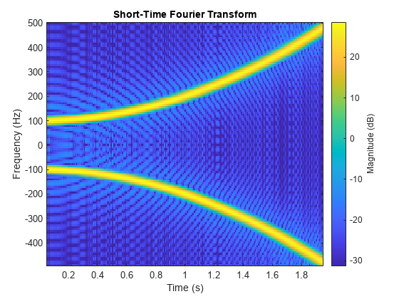
Generate a signal consisting of a chirp sampled at 1.4 kHz for 2 seconds. The frequency of the chirp decreases linearly from 600 Hz to 100 Hz during the measurement time.
fs = 1400;
x = chirp(0:1/fs:2,600,2,100);
stft Defaults
Compute the STFT of the signal using the spectrogram and stft functions. Use the default values of the stft function:
Divide the signal into 128-sample segments and window each segment with a periodic Hann window.
Specify 96 samples of overlap between adjoining segments. This length is equivalent to 75% of the window length.
Specify 128 DFT points and center the STFT at zero frequency, with the frequency expressed in hertz.
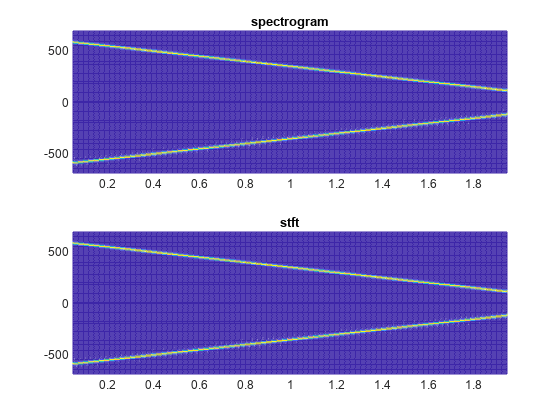
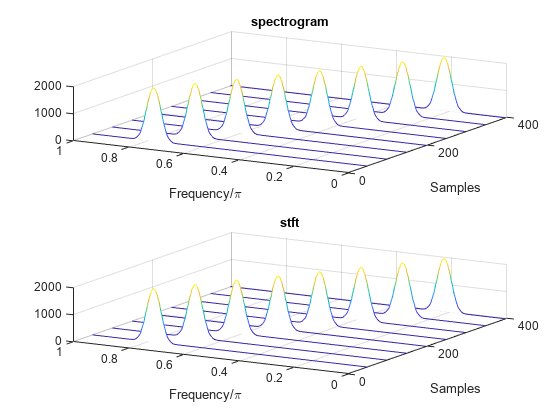
Verify that the two results are equal.
M = 128;
g = hann(M,"periodic");
L = 0.75*M;
Ndft = 128;

[sp,fp,tp] = spectrogram(x,g,L,Ndft,fs,"centered");

[s,f,t] = stft(x,fs);

dff = max(max(abs(sp-s)))
dff =
0
Use the mesh function to plot the two outputs.
nexttile
mesh(tp,fp,abs(sp).^2)
title("spectrogram")
view(2), axis tight

nexttile
mesh(t,f,abs(s).^2)
title("stft")
view(2), axis tight
spectrogram Defaults
Repeat the computation using the default values of the spectrogram function:
Divide the signal into segments of length , where is the length of the signal. Window each segment with a Hamming window.
Specify 50% overlap between segments.
To compute the FFT, use points. Compute the spectrogram only for positive normalized frequencies.
M = floor(length(x)/4.5);
g = hamming(M);
L = floor(M/2);
Ndft = max(256,2^nextpow2(M));

[sx,fx,tx] = spectrogram(x);

[st,ft,tt] = stft(x,Window=g,OverlapLength=L, ...
    FFTLength=Ndft,FrequencyRange="onesided");

dff = max(max(sx-st))
dff =
0
Use the waterplot function to plot the two outputs. Divide the frequency axis by in both cases. For the stft output, divide the sample numbers by the effective sample rate, .
figure
nexttile
waterplot(sx,fx/pi,tx)
title("spectrogram")

nexttile
waterplot(st,ft/pi,tt/(2*pi))
title("stft")
function waterplot(s,f,t)
% Waterfall plot of spectrogram
    waterfall(f,t,abs(s)'.^2)
    set(gca,XDir="reverse",View=[30 50])
    xlabel("Frequency/\pi")
    ylabel("Samples")
end
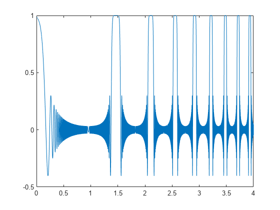
Generate a signal sampled at 5 kHz for 4 seconds. The signal consists of a set of pulses of decreasing duration separated by regions of oscillating amplitude and fluctuating frequency with an increasing trend. Plot the signal.
fs = 5000;
t = 0:1/fs:4-1/fs;

x = besselj(0,600*(sin(2*pi*(t+1).^3/30).^5));

plot(t,x)
Compute the one-sided, two-sided, and centered short-time Fourier transforms of the signal. In all cases, use a 202-sample Kaiser window with shape factor to window the signal segments. Display the frequency range used to compute each transform.
rngs = ["onesided" "twosided" "centered"];

for kj = 1:length(rngs)

    opts = {"Window",kaiser(202,10),"FrequencyRange",rngs(kj)};

    [~,f] = stft(x,fs,opts{:});
    subplot(length(rngs),1,kj)
    stft(x,fs,opts{:})
    title(sprintf('''%s'': [%5.3f, %5.3f] kHz',rngs(kj),[f(1) f(end)]/1000))

end
![Figure contains 3 axes objects. Axes object 1 with title 'onesided': [0.000, 2.500] kHz, xlabel Time (s), ylabel Frequency (kHz) contains an object of type image. Axes object 2 with title 'twosided': [0.000, 4.975] kHz, xlabel Time (s), ylabel Frequency (kHz) contains an object of type image. Axes object 3 with title 'centered': [-2.475, 2.500] kHz, xlabel Time (s), ylabel Frequency (kHz) contains an object of type image.](../../examples/signal/win64/STFTFrequencyRangesExample_02.png)
Repeat the computation, but now change the length of the Kaiser window to 203, an odd number. The "twosided" frequency interval does not change. The other two frequency intervals become open at the higher end.
for kj = 1:length(rngs)

    opts = {"Window",kaiser(203,10),"FrequencyRange",rngs(kj)};

    [~,f] = stft(x,fs,opts{:});
    subplot(length(rngs),1,kj)
    stft(x,fs,opts{:})
    title(sprintf('''%s'': [%5.3f, %5.3f] kHz',rngs(kj),[f(1) f(end)]/1000))

end
![Figure contains 3 axes objects. Axes object 1 with title 'onesided': [0.000, 2.488] kHz, xlabel Time (s), ylabel Frequency (kHz) contains an object of type image. Axes object 2 with title 'twosided': [0.000, 4.975] kHz, xlabel Time (s), ylabel Frequency (kHz) contains an object of type image. Axes object 3 with title 'centered': [-2.488, 2.488] kHz, xlabel Time (s), ylabel Frequency (kHz) contains an object of type image.](../../examples/signal/win64/STFTFrequencyRangesExample_03.png)
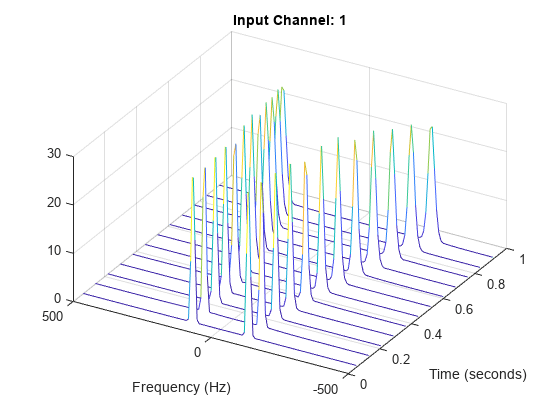
Generate a three-channel signal consisting of three different chirps sampled at 1 kHz for one second.
The first channel consists of a concave quadratic chirp with instantaneous frequency 100 Hz at t = 0 and crosses 300 Hz at t = 1 second. It has an initial phase equal to 45 degrees.
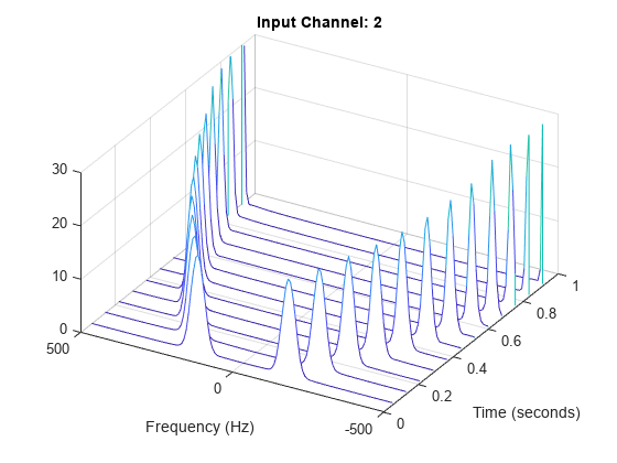
The second channel consists of a convex quadratic chirp with instantaneous frequency 100 Hz at t = 0 and crosses 500 Hz at t = 1 second.
The third channel consists of a logarithmic chirp with instantaneous frequency 300 Hz at t = 0 and crosses 500 Hz at t = 1 second.
Compute the STFT of the multichannel signal using a periodic Hamming window of length 128 and an overlap length of 50 samples.
fs = 1e3;
t = 0:1/fs:1-1/fs;

x = [chirp(t,100,1,300,"quadratic",45,"concave");
      chirp(t,100,1,500,"quadratic",[],"convex");
      chirp(t,300,1,500,"logarithmic")]';

[S,F,T] = stft(x,fs,Window=hamming(128,"periodic"),OverlapLength=50);
Visualize the STFT of each channel as a waterfall plot. Control the behavior of the axes using the helper function helperGraphicsOpt.
waterfall(F,T,abs(S(:,:,1))')
helperGraphicsOpt(1)
waterfall(F,T,abs(S(:,:,2))')
helperGraphicsOpt(2)
waterfall(F,T,abs(S(:,:,3))')
helperGraphicsOpt(3)
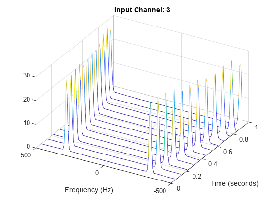
This helper function sets the appearance and behavior of the current axes.
function helperGraphicsOpt(ChannelId)
ax = gca;
ax.XDir = "reverse";
ax.ZLim = [0 30];
ax.Title.String = "Input Channel: " + ChannelId;
ax.XLabel.String = "Frequency (Hz)";
ax.YLabel.String = "Time (seconds)";
ax.View = [30 45];
end
Since R2026a
Plot the magnitude-squared STFT for four signals in the specified target axes and panel containers.
Create four oscillating signals with a sample rate of 10 kHz for three seconds.
Fs = 10e3;
t = 0:1/Fs:3;
x1 = vco(sawtooth(2*pi*t,0.5),[0.1 0.4]*Fs,Fs);
x2 = vco(sin(2*pi*t).*exp(-t),[0.1 0.4]*Fs,Fs) ...
    + 0.01*sin(2*pi*0.25*Fs*t);
x3 = exp(1j*pi*sin(4*t)*Fs/10);
x4 = chirp(t,Fs/10,t(end),Fs/2.5,"quadratic");
Plot STFT in Target Axes
Create two axes in the southwestern and northeastern corners of a new figure window.
fig = figure;
ax1 = axes(fig,Position=[0.08 0.1 0.55 0.45]);
ax2 = axes(fig,Position=[0.48 0.7 0.48 0.25]);
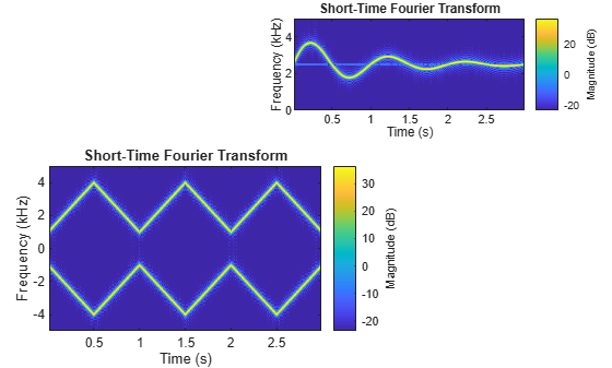
Plot the magnitude-squared STFT of the signals x1 and x2 in the southwestern and northeastern axes of the figure, respectively. Display a one-sided frequency range for the STFT of x2. Use a 256-sample Kaiser window, an overlap length of 220 samples, and 512 DFT points.
g = kaiser(256,5);
ol = 220;
nfft = 512;

stft(x1,Fs,Window=g,OverlapLength=ol,FFTLength=nfft,Parent=ax1)
stft(x2,Fs,Window=g,OverlapLength=ol,FFTLength=nfft, ...
    FrequencyRange="onesided",Parent=ax2)
Plot STFT in Target UI Axes
Create an axes in the northwestern corner of a new UI figure window.
uif = uifigure(Position=[100 100 720 540]);
ax3 = uiaxes(uif,Position=[5 305 300 200]);
Plot the magnitude-squared STFT of the signal x3 on the figure axes.
stft(x3,Fs,Window=g,OverlapLength=ol,FFTLength=nfft,Parent=ax3)
title(ax3,"STFT in UI Axes")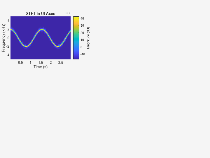
Plot STFT in Target Panel Container
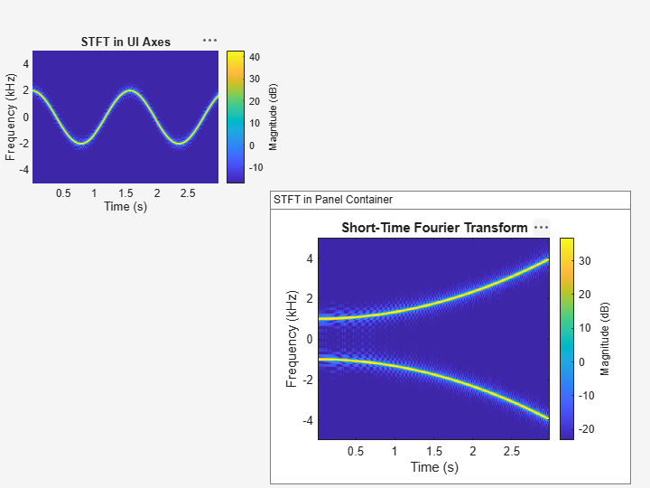
Add a panel container in the southeastern corner of the UI figure window.
p = uipanel(uif,Position=[300 5 400 325], ...
    Title="STFT in Panel Container", ...
    BackgroundColor="white");
Plot the magnitude-squared STFT of the signal x4 on the panel container.
stft(x4,Fs,Window=g,OverlapLength=ol,FFTLength=nfft,Parent=p)
Input Arguments
Name-Value Arguments
Output Arguments
More About
References
[1] Mitra, Sanjit K. Digital Signal Processing: A Computer-Based Approach. 2nd Ed. New York: McGraw-Hill, 2001.
[2] Sharpe, Bruce. Invertibility of Overlap-Add Processing. https://gauss256.github.io/blog/cola.html, accessed July 2019.
[3] Smith, Julius Orion. Spectral Audio Signal Processing. https://ccrma.stanford.edu/~jos/sasp/, online book, 2011 edition, accessed Nov 2018.