sbioplot

Plot simulation results in one figure

Syntax

sbioplot(sd)

sbioplot(sd,fcnHandle,xArgs,yArgs,Name,Value)

Description

sbioplot(sd) plots each simulation run from sd, a SimData object or array of objects, in the same figure. The plot is a time plot of each state in sd. The figure also shows a hierarchical display of all the runs as different nodes in a tree, and you can select which run to display.

sbioplot(sd,fcnHandle,xArgs,yArgs,Name,Value) plots simulation results by calling the function handle fcnHandle with inputs sd, xArgs, and yArgs, and uses additional options specified by one or more name-value pair arguments. For example, you can specify the x-label and y-label of the plot. xArgs and yArgs must be cell arrays or string vectors of the names of the states to plot.

Examples

Plot Selected States from Simulation Data

Plot the prey versus predator data from the stochastically simulated lotka model by using a custom function (plotXY).

Load the model. Set the solver type to SSA to perform stochastic simulations, and set the stop time to 3.

sbioloadproject lotka;
cs              = getconfigset(m1);
cs.SolverType   = 'SSA';
cs.StopTime     = 3;
rng('default') % For reproducibility

Set the number of runs and use sbioensemblerun for simulation.

numRuns = 2;
sd      = sbioensemblerun(m1,numRuns);

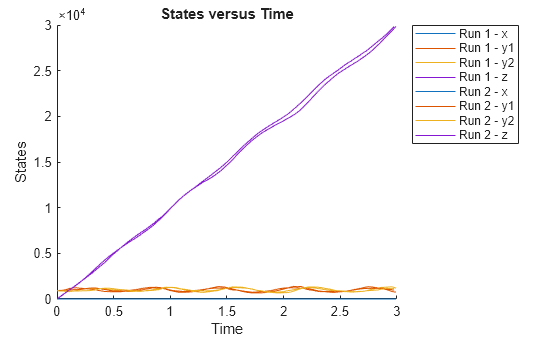
Plot the simulation data. By default, sbioplot shows the time plot of each species for each run. You can expand each run by clicking the + icon, and you can select individual time plots.

sbioplot(sd); 

Plot selected states against each other; in this case, plot the prey population versus the predator population. Use the function plotXY (shown at the end of this example) to plot the simulated y1 (prey) data versus the y2 (predator) data. Specify the function as a function handle.

If you use the live script file for this example, the plotXY function is already included at the end of the file. Otherwise, you must define the plotXY function at the end of your .m or .mlx file or add it as a file on the MATLAB path.

sbioplot(sd,@plotXY,{'y1'},{'y2'},'xlabel','y1','ylabel','y2','title','Prey versus Predator');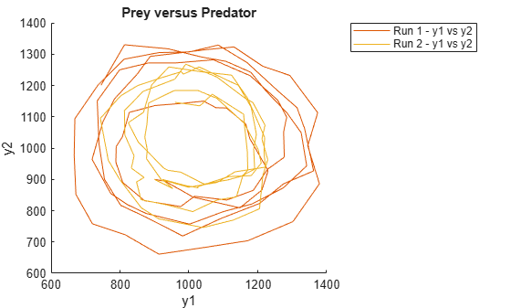

Define plotXY Function

sbioplot accepts a function handle for a function with the signature:

function [handles,names] = functionName(sd,xArgs,yArgs).

The plotXY function plots two selected states against each other. The first input sd is the simulation data (SimBiology SimData object or vector of objects). In this particular example, xArgs is a cell array containing the name of the species to be plotted on the x-axis, and yArgs is a cell array containing the name of the second species to be plotted on the y-axis. However, you can use the inputs xArgs and yArgs in any way in your custom plotting function. The function returns handles, an array of function handles to the line plots, and names, a cell array of character vectors shown on the nodes that are children of a Run node in a hierarchical display.

function [handles,names] = plotXY(sd,xArgs,yArgs)
    
% Select simulation data for each state from each run.
xData1 = selectbyname(sd(1),xArgs);
xData2 = selectbyname(sd(2),xArgs);
yData1 = selectbyname(sd(1),yArgs);
yData2 = selectbyname(sd(2),yArgs);

% Plot the species against each other.
fH1 = plot(xData1.Data,yData1.Data);
fH2 = plot(xData2.Data,yData2.Data);

% The first output, handles, is a two-dimensional array of handles of the line plots. It must be of size M x N, 
% where M is the number of line plots for each run and N is the number of runs.
handles = [fH1,fH2];

% The second output, names, must be a one-dimensional cell array of character vectors.
% Its length must be equal to the number of rows in handles, and the texts are displayed on the 
% nodes that are children of a Run node.
names = {'y1 vs y2'};
   
end

Input Arguments

sd — Simulation results

SimData object

Simulation results, specified as a SimData object or vector of SimData objects.

This argument corresponds to the first input of the function referenced by fcnHandle.

Example: simdata

fcnHandle — Function to generate line plots

function handle

Function to generate line plots, specified as a function handle. For an example of a custom function to plot selected species from simulation data, see Plot Selected States from Simulation Data.

The function must have the signature:

function [handles,names] = functionName(sd,xArgs,yArgs).

The inputs sd, xArgs, and yArgs are the same inputs that you pass in when you call sbioplot.

The first output handles is a two-dimensional array of handles of the line plots generated by the function. Its size must be P-by-R, where P is the number of line plots, and R is the number of runs.

The second output names is a one-dimensional cell array of character vectors containing the names to be displayed on the nodes that are children of a Run node in a hierarchical display. The length of names must be equal to the number of rows in handles.

Example: @plotXY

Data Types: function_handle

xArgs — State names

string vector | cell array of character vectors

State names to plot, specified as a string vector or cell array of character vectors. For instance, you can use xArgs to represent the states to be plotted on the x-axis of your custom plot.

This argument corresponds to the second input of the function referenced by fcnHandle.

Example: {'y1'}

Data Types: cell

yArgs — State names

string vector | cell array of character vectors

State names to plot, specified as a string vector or cell array of character vectors. For instance, you can use yArgs to represent the states to be plotted on the y-axis of your custom plot.

This argument corresponds to the third input of the function referenced by fcnHandle.

Example: {'y2','z'}

Data Types: cell

Name-Value Pair Arguments

Specify optional comma-separated pairs of Name,Value arguments. Name is the argument name and Value is the corresponding value. Name must appear inside quotes. You can specify several name and value pair arguments in any order as Name1,Value1,...,NameN,ValueN.

Example: 'title','Species X versus Species Y' specifies the axes title of the plot.

'title' — Axes title

character vector | string

Axes title, specified as the comma-separated pair consisting of 'title' and character vector or string.

Example: 'title','Prey versus Predator'

Data Types: char | string

'xlabel' — Label for x-axis

character vector | string

Label for the x-axis of the plot, specified as the comma-separated pair consisting of 'xlabel' and a character vector or string.

Example: 'xlabel','y1'

Data Types: char | string

'ylabel' — Label for y-axis

character vector | string

Label for the y-axis of the plot, specified as the comma-separated pair consisting of 'ylabel' and a character vector or string.

Example: 'ylabel','y2'

Data Types: char | string