Model an Automatic Transmission Controller
This example shows how to model an automotive drivetrain using Simulink®. In this model, a Stateflow® chart implements the transmission control logic and integrates directly with the Simulink model, combining control logic and drivetrain dynamics in a clear and intuitive structure.
Model Analysis and Physics
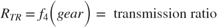
This figure shows the power flow in a typical automotive drivetrain. The model uses nonlinear ordinary differential equations to simulate the engine, four-speed automatic transmission, and vehicle dynamics. The model implements each component from the diagram as a modular Simulink subsystem. In contrast, the transmission control unit logic does not translate easily into mathematical equations. Instead, the model uses a Stateflow chart to represent the TCU. The Stateflow chart monitors key system events and responds immediately by executing the appropriate gear selection logic.
![]()
The throttle opening is one of the inputs to the engine. The engine is connected to the impeller of the torque converter, which couples it to the transmission, as shown in Equation Set 1.
Equation Set 1


The model implements the input-output characteristics of the torque converter as functions of the engine and turbine speed. The direction of power flows from the impeller to the turbine, as shown in Equation Set 2.
Equation Set 2


The model implements the transmission via static gear ratios, assuming small shift times, as shown in Equation Set 3.
Equation Set 3


The final drive, inertia, and a dynamically varying load constitute the vehicle dynamics, as shown in Equation Set 4.
Equation Set 4


The load torque includes both the road load and brake torque. The road load is the sum of frictional and aerodynamic losses, as shown in Equation Set 5.
Equation Set 5


This model implements the transmission shift points based on the schedule, as shown in this figure. For each gear and throttle setting, the model defines a unique vehicle speed that triggers an upshift. The simulation applies the same logic for downshifts.
![]()
Opening and Simulating the Model
Opening the model sets the initial conditions in the model workspace.
To run the simulation, on the Simulation tab, click Run. The model logs relevant data to the MATLAB Workspace in a structure named sldemo_autotrans_output. Logged signals are marked with a blue indicator. After the simulation completes, you can view the contents of the data structure by entering sldemo_autotrans_output in the MATLAB Command Window. The model also displays units on subsystem icons and signal lines for clarity.
![]()
The Simulink model organizes the drivetrain into modular components that represent the engine, transmission, and vehicle. A dedicated shift logic block controls the transmission ratio. The model accepts user inputs in the form of throttle (percent) and brake torque (ft-lb), which you can specify by setting parameter values for the Signal Editor block named ManeuversGUI.
The Engine subsystem uses a two-dimensional lookup table to interpolate engine torque based on throttle and engine speed. To explore the structure, double-click the subsystem.
![]()
The Transmission subsystem contains the TorqueConverter and the TransmissionRatio blocks. To view the components, double-click the Transmission subsystem.
![]()
TorqueConverter is a masked subsystem that implements Equation Set 2. To open this subsystem, right-click and select Edit Mask > Look Inside Mask. The mask requires a vector of speed ratios (Nin/Ne) and vectors of K-factor (f2) and torque ratio (f3).
![]()
The transmission ratio block determines the ratio shown in the table, and then uses Equation Set 3 to compute the transmission output torque and input speed.
Table: Transmission Gear Ratios
Gear     Rtr = Nin/Ne
 1         2.393
 2         1.450
 3         1.000
 4         0.677
![]()
The Stateflow chart ShiftLogic implements the gear selection in the transmission. To open the Stateflow chart, double-click ShiftLogic. In the Model Explorer, you can define throttle and vehicle speed as inputs and set the desired gear number as the output. Two dashed AND states track the current gear and the gear selection process. The chart runs as a discrete-time system, sampled every 40 milliseconds.
![]()
To see how the shift logic behaves during simulation, enable animation in the Stateflow debugger. The always-active selection_state starts by executing its during function, which calculates upshift and downshift speed thresholds based on the current gear and throttle input. While in the steady_state, the model compares these thresholds to the vehicle speed to decide whether a shift is needed. If a shift is required, the model enters either the upshifting or downshifting confirm state and records the entry time.
If the vehicle speed no longer meets the shift condition while in a confirm state, the model cancels the shift and returns to the steady_state state. This logic prevents unnecessary shifts caused by noise. If the shift condition holds for TWAIT ticks, the model transitions through the lower junction and broadcasts a shift event based on the current gear. It then reactivates state via a central junction. The shift event, which is broadcast to the gear_selection state, activates a transition to the appropriate new gear.
For example, if the vehicle runs in second gear with 25% throttle, the second state is active in gear_state, and steady_state state is active in selection_state. The during function determines that an upshift should occur when the vehicle exceeds 30 mph. Once this condition is met, the model enters the upshifting state. If the speed stays above 30 mph for TWAIT ticks, the model transitions through the lower right junction, satisfies the condition gear == 2, and moves from upshifting to the steady_state state, broadcasting the UP event. This event causes the gear to shift from second to third in gear_state, completing the logic.
Vehicle is a masked subsystem that uses net torque to calculate acceleration and integrates it to determine vehicle speed, per Equation Sets 4 and 5. To look under the mask, right-click the Vehicle block and select Edit Mask > Look Inside Mask. In the mask menu, you can enter parameters such as final drive ratio, drag friction and aerodynamic drag coefficients, wheel radius, vehicle inertia, and initial transmission output speed.
![]()
Results
During simulation, the model implements this engine torque map and torque converter characteristics.
![]()
This figure shows the FactorK and the TorqueRatio versus SpeedRatio.
![]()
The first simulation is a passing maneuver and uses the throttle schedule given in this table. The model interpolates this data linearly.
Table: Throttle schedule for Passing Maneuver
Time (sec)    Throttle (%)
  0             60
 14.9           40
 15            100
 100            0
 200            0
The first column corresponds to time. The second column corresponds to throttle opening in percent. In this case, no brake is applied, and brake torque is zero. The vehicle speed starts at zero and the engine at 1000 RPM. This figure shows the plot for the baseline results, using the default parameters. As the driver steps to 60% throttle at t = 0, the engine immediately responds by more than doubling its speed. This increase brings about a low speed ratio across the torque converter and a large torque ratio. The vehicle accelerates quickly, and the tire does not slip. Both the engine and the vehicle gain speed until approximately t = 2 sec, at which time a 1 to 2 upshift occurs. The engine speed characteristically drops abruptly, then resumes its acceleration. The 2 to 3 and 3 to 4 upshifts take place at about four and eight seconds, respectively. The vehicle speed remains much smoother due to its large inertia.
![]()
At t = 15 sec, the driver steps the throttle to 100%, as might be typical of a passing maneuver. The transmission downshifts to third gear, and the engine jumps from about 2600 RPM to about 3700 RPM. The engine torque increases, which increases the mechanical advantage of the transmission. With continued heavy throttle, the vehicle accelerates to about 100 mph and then shifts into overdrive at about t = 21 sec. The vehicle cruises along in fourth gear for the remainder of the simulation. Double-click the ManeuversGUI block and change parameter values to vary the throttle and brake history.
Running Multiple Scenarios and Collecting Coverage
You can run the model for all scenarios while collecting coverage. To see a saved design study for running all of the scenarios of sldemo_autotrans, open the Multiple Simulations panel. In the Prepare section of the Simulink Toolstrip, in the Inputs & Parameter Tuning section, click Multiple Simulations. Then, open the sldemo_autotrans_design_study.mldatx design file.
After you open the design study, use these commands to enable the model coverage and cumulative collection in the model settings.
set_param('sldemo_autotrans', 'CovEnable', 'on'); set_param('sldemo_autotrans', 'CovEnableCumulative', 'on');
Then, check model coverage of the design cases.