Mark Signals of Interest for Batch Linearization
When batch linearizing a model using an slLinearizer interface, you can mark signals of interest using analysis
points. You can then analyze the response of your system at any of these points using
functions such as getIOTransfer and getLoopTransfer.
Alternatively, if you are batch linearizing your model using the:
Model Linearizer, specify analysis points as shown in Specify Portion of Model to Linearize in Model Linearizer.
For more information on selecting a batch linearization tool, see Choose Batch Linearization Methods.
Analysis Points
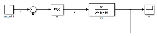
Analysis points identify locations within a Simulink® model that are relevant for linear analysis. Each analysis point is
associated with a signal that originates from the outport of a Simulink block. For example, in the following model, the reference signal
r and the control signal u are analysis points
that originate from the outputs of the setpoint and C
blocks respectively.
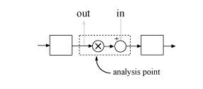
Each analysis point can serve one or more of the following purposes:
Input — The software injects an additive input signal at an analysis point, for example, to model a disturbance at the plant input.
Output — The software measures the signal value at a point, for example, to study the impact of a disturbance on the plant output.
Loop Opening — The software interprets a break in the signal flow at a point, for example, to study the open-loop response at the plant input.
When you use an analysis point for more than one purpose, the software applies the purposes in this sequence: output measurement, then loop opening, then input.
Using analysis points, you can extract open-loop and closed-loop responses from a Simulink model. You can also specify requirements for control system tuning using analysis points. For more information, see Mark Signals of Interest for Control System Analysis and Design.
Specify Analysis Points
You can mark analysis points either explicitly in the Simulink model, or programmatically using the addPoint command for an slLinearizer
interface.
Mark Analysis Points in Simulink Model
To specify analysis points directly in your Simulink model, first open the Linearization tab. To do so, in the Apps gallery, click Linearization Manager.
To specify an analysis point:
In the model, click the signal you want to define as an analysis point.
On the Linearization tab, in the Insert Analysis Points gallery, select the type of analysis point you want to define.
When you specify analysis points, the software adds annotations to your model indicating the linear analysis point type.
Repeat steps 1 and 2 for all signals you want to define as analysis points.
You can select any of the following closed-loop analysis point types, which are
equivalent within an slLinearizer interface.
Input Perturbation
Output Measurement
Sensitivity
Complementary Sensitivity
If you want to introduce a permanent loop opening at a signal as well, select one of the following open-loop analysis point types:
Open-Loop Input
Open-Loop Output
Loop Transfer
Loop Break
When you define a signal as an open-loop point, analysis functions such as
getIOTransfer always enforce a loop break at that signal
during linearization. All open-loop analysis point types are equivalent within an
slLinearizer interface. For more information on how the
software treats loop openings during linearization, see How the Software Treats Loop Openings.
When you create an slLinearizer interface for a model, any
analysis points defined in the model are automatically added to the interface. If you
defined an analysis point using:
A closed-loop type, the signal is added as an analysis point only.
An open-loop type, the signal is added as both an analysis point and a permanent opening.
Mark Analysis Points Programmatically
To mark analysis points programmatically, use the addPoint command. For example, consider the scdcascade model.
open_system('scdcascade')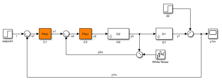
To mark analysis points, first create an slLinearizer interface.
sllin = slLinearizer('scdcascade');To add a signal as an analysis point, use the addPoint command, specifying the source block and port number for the signal.
addPoint(sllin,'scdcascade/C1',1);If the source block has a single output port, you can omit the port number.
addPoint(sllin,'scdcascade/G2');For convenience, you can also mark analysis points using the:
Name of the signal.
addPoint(sllin,'y2');Combined source block path and port number.
addPoint(sllin,'scdcascade/C1/1')End of the full source block path when unambiguous.
addPoint(sllin,'G1/1')You can also add permanent openings to an slLinearizer interface using the addOpening command, and specifying signals in the same way as for addPoint. For more information on how the software treats loop openings during linearization, see How the Software Treats Loop Openings.
addOpening(sllin,'y1m');You can also define analysis points by creating linearization I/O objects using the linio command.
io(1) = linio('scdcascade/C1',1,'input');
io(2) = linio('scdcascade/G1',1,'output');
addPoint(sllin,io);
As when you define analysis points directly in your model, if you specify a linearization I/O object with:
A closed-loop type, the signal is added as an analysis point only.
An open-loop type, the signal is added as both an analysis point and a permanent opening.
Refer to Analysis Points
Once you have marked analysis points in an slLinearizer
interface, you can analyze the response at any of these points using the following
analysis functions:
getIOTransfer— Transfer function for specified inputs and outputsgetLoopTransfer— Open-loop transfer function from an additive input at a specified point to a measurement at the same pointgetSensitivity— Sensitivity function at a specified pointgetCompSensitivity— Complementary sensitivity function at a specified point
To view the available analysis points in an slLinearizer
interface, use the getPoints command.
See Also
addPoint | getPoints | slLinearizer | addOpening