Planar Contact Force

Libraries:
Simscape /
Multibody /
Forces and Torques
Description
The Planar Contact Force block models the planar contact between these geometry pairs:
Disk and disk
Disk and line segment
Disk and point
Disk and 2-D point cloud
When modeling planar contacts, the two geometries must be coplanar and the z-axes of the base and follower geometries must be aligned and point to the same direction.
Contacts
You can use the built-in penalty method or provide custom normal and friction force laws to model a contact. The Planar Contact Force block uses the same penalty method as the Spatial Contact Force block, but with the normal force along the y-axis of the contact frame and the friction force along the x-axis of the contact frame. For more information about the penalty model, see Contact Forces.
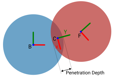
When modeling contacts between two disks or a disk and a line segment, there is a single contact point located at the center of the penetration depth. Each geometry has one contact frame. The two frames are always coincident and located at the contact point. The positive y-axis of the contact frame is aligned with the contact normal direction pointing from the base geometry to the follower geometry, and the z-axis is aligned with the z-axis of the base frame. The image shows the contact between two disks. The B, F, and C frames are the base, follower, and contact frames, respectively.
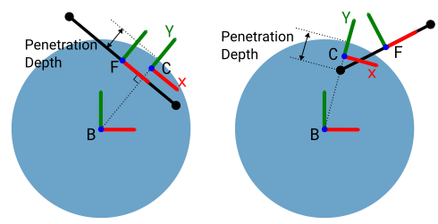
This image shows two scenarios that show contact between a disk and a line segment.
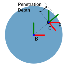
When modeling contacts between a disk and a point, there is a single contact point that is coincident with the point.
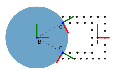
When modeling contacts between a disk and a 2-D point cloud, there is a contact point for each point that is in contact with the disk. The Planar Contact Force block computes the contact quantities for each point and the output signals have the same order as the points specified in the Point Could block. For the points that are not in contact with the disk, the measured values are zero. When using input forces, the size and order of the input signals must match the size and order of the points specified in the Point Could block.
Ports
Geometry
Geometry port associated with the base geometry.
Geometry port associated with the follower geometry.
Input
Physical signal input port that accepts the normal contact force magnitude between the two geometries. The block clips negative values to zero.
When modeling contacts that involve a point cloud, the input signal must be a 1-by-N array, where N equals the number of points. Each column of the array specifies the normal contact force on one of the points. The size and order of the input signals must match the size and order of the points specified in the Point Could block. The force is resolved in the contact frame of the point.
When modeling contacts between other types of geometries, the input signal must be a scalar that specifies the normal contact force.
Dependencies
To enable this port, in the Normal Force section, set
Method to Provided by
Input.
Physical signal input port that accepts the frictional force between the two geometries.
When modeling contacts that involve a point cloud, the input signal must be a 1-by-N array, where N equals the number of points. Each column of the array specifies the x-component of the applied frictional force on one of the points. The size and order of the input signals must match the size and order of the points specified in the Point Could block. The force is resolved in the contact frame of the point.
When modeling contacts between other types of geometries, the input signal must be a scalar that specifies the x-component of the applied frictional force resolved in the contact frame.
Dependencies
To enable this port, in the Frictional Force section, set
Method to Provided by
Input.
Output
Physical signal output port that outputs the contact status of the two geometries.
When modeling contacts that involve a point cloud, the output is a 1-by-N array, where N equals the number of points. Each column of the array indicates the status of the corresponding point. The point contacts the other geometry if the output is 1. Otherwise, the output is 0.
When modeling contacts between other types of geometries, the output is a scalar that indicates whether the geometries are in contact. The geometries are in contact if the output is 1 or separated if the output is 0.
Dependencies
To enable this port, in the Sensing section, select Contact Signal.
Physical signal output port that outputs the penetration depth between the two geometries.
When modeling contacts that involve a point cloud, the output is a 1-by-N array, where N equals the number of points. Each column of the array indicates the status of the corresponding point. If the point is penetrating the other geometry, the output is positive and equals the penetration depth. Otherwise, the output is 0.
When modeling contacts between other types of geometries, the output is a scalar that indicates whether the geometries are penetrating each other. If they are penetrating each other, the output is positive and equals the penetration depth. Otherwise, the output is 0.
Dependencies
To enable this port, in the Sensing section, select Penetration Depth.
Physical signal output port that outputs the relative normal velocity between the contact points of the base and follower geometries.
When modeling contacts that involve a point cloud, the output is a 1-by-N array, where N equals the number of points. Each column of the array equals the y-component of the relative velocity between the corresponding point and the contact point on the other geometry. The relative velocity is resolved in the corresponding contact frame.
When modeling contacts between other types of geometries, the output is a scalar that equals the y-component of the relative velocity between the contact points of the two geometries. The output is resolved in the contact frame.
Dependencies
To enable this port, in the Sensing section, select Relative Normal Velocity.
Physical signal output port that outputs the relative tangential velocity between the contact points of the base and follower geometries.
When modeling contacts that involve a point cloud, the output is a 1-by-N matrix, where N equals the number of points. Each column of the array equals the x-component of the relative velocity between the corresponding point and the contact point on the other geometry. The relative velocity is resolved in the corresponding contact frame.
When modeling contacts between other types of geometries, the output is a scalar that equals the x-component of the relative velocity between the contact points of the two geometries. The output is resolved in the contact frame.
Dependencies
To enable this port, in the Sensing section, select Relative Tangential Velocity.
Force/Torque
Physical signal output port for the normal force between two contact geometries. The block resolves the measurement in the coordinates of the specified resolution frame, and the setting of the Direction parameter affects the sign of the measurement.
When modeling contacts that involve a point cloud, the output is a 3-by-N array, where N represents the number of points. Each column of the array represents a 3-D vector that indicates the normal force at the corresponding point.
When modeling contacts between other types of geometries, the output represents a 3-D vector that indicates the normal force.
Dependencies
To enable this port, in the Force/Torque section, select Normal Force.
Physical signal output port for the magnitude of the normal force. The Direction and Resolution Frame parameters do not affect the measurement.
When modeling contacts that involve a point cloud, the output is a 1-by-N array, where N equals the number of points. Each column of the array is the magnitude of the normal force at the corresponding point.
When modeling contacts between other types of geometries, the output is the magnitude of the normal force.
Dependencies
To enable this port, in the Force/Torque section, select Normal Force Magnitude.
Physical signal output port for the torque resulting from the normal force. The measurement is the cross product of the normal force and the position vector of the contact point relative to the specified resolution frame. The Direction parameter affects the sign of the measurement.
When modeling contacts that involve a point cloud, the output is a 3-by-N array, where N represents the number of points. Each column of the array represents a 3-D vector that indicates the torque due to the normal force at the corresponding point.
When modeling contacts between other types of geometries, the output represents a 3-D vector that indicates the torque due to the normal force.
Dependencies
To enable this port, in the Force/Torque section, select Normal Torque.
Physical signal output port for the frictional force between two contact geometries. The block resolves the measurement in the coordinates of the specified resolution frame, and the setting of the Direction parameter affects the sign of the measurement.
When modeling contacts that involve a point cloud, the output is a 3-by-N array, where N represents the number of points. Each column of the array represents a 3-D vector that indicates the frictional force at the corresponding point.
When modeling contacts between other types of geometries, the output represents a 3-D vector that indicates the frictional force.
Dependencies
To enable this port, in the Force/Torque section, select Frictional Force.
Physical signal output port for the magnitude of the frictional force between two contact geometries. The Direction and Resolution Frame parameters do not affect the measurement.
When modeling contacts that involve a point cloud, the output is a 1-by-N array, where N equals the number of points. Each column of the array is the magnitude of the frictional force at the corresponding point.
When modeling contacts between other types of geometries, the output is the magnitude of the normal contact force.
Dependencies
To enable this port, in the Force/Torque section, select Frictional Force Magnitude.
Physical signal output port for the torque resulting from the frictional force. The measurement is the cross product of the frictional force and the position vector of the contact point relative to the specified resolution frame. The Direction parameter affects the sign of the measurement.
When modeling contacts that involve a point cloud, the output is a 3-by-N array, where N represents the number of points. Each column of the array represents a 3-D vector that indicates the torque due to the frictional force at the corresponding point.
When modeling contacts between other types of geometries, the output represents a 3-D vector that indicates the torque due to the frictional force.
Dependencies
To enable this port, in the Force/Torque section, select Frictional Torque.
Physical signal output port for the total contact force between two contact geometries. The total contact force includes normal and frictional forces. The block resolves the measurement in the coordinates of the specified resolution frame, and the setting of the Direction parameter affects the sign of the measurement.
When modeling contacts that involve a point cloud, the output is a 3-by-N array, where N represents the number of points. Each column of the array represents a 3-D vector that indicates the total contact force at the corresponding point.
When modeling contacts between other types of geometries, the output represents a 3-D vector that indicates the total contact force.
Dependencies
To enable this port, in the Force/Torque section, select Total Force.
Physical signal output port for the total contact torque resulting from the contact force. The measurement is the cross product of the contact force and the position vector of the contact point relative to the specified resolution frame. The Direction parameter affects the sign of the measurement.
When modeling contacts that involve a point cloud, the output is a 3-by-N array, where N represents the number of points. Each column of the array represents a 3-D vector that indicates the contact torque due to the total contact force at the corresponding point.
When modeling contacts between other types of geometries, the output represents a 3-D vector that indicates the torque due to the total contact force.
Dependencies
To enable this port, in the Force/Torque section, select Total Torque.
Contact Frame
Physical signal port that outputs a 3-by-3 rotation matrix that maps the vectors in the contact frame to vectors in the reference frame of the base geometry. The output signal is resolved in the reference frame associated with the base geometry.
Dependencies
To enable this port, in the Sensing > Contact Frame section, select Base Rotation.
Physical signal port that outputs a 3-by-1 vector that contains the coordinates of the origin of the contact frame resolved in the reference frame of the base geometry.
Dependencies
To enable this port, in the Sensing > Contact Frame section, select Base Translation.
Physical signal port that outputs a 3-by-3 rotation matrix that maps vectors in the contact frame to vectors in the reference frame of the follower geometry. The output signal is resolved in the reference frame associated with the follower geometry.
Dependencies
To enable this port, in the Sensing > Contact Frame section, select Follower Rotation.
Physical signal port that outputs a 3-by-1 vector that contains the coordinates of the origin of the contact frame resolved in the reference frame of the follower geometry.
Dependencies
To enable this port, in the Sensing > Contact Frame section, select Follower Translation.
Parameters
Normal Force
Method to specify the normal contact force, specified as either
Smooth Spring-Damper or Provided by
Input.
Select Smooth Spring-Damper to use the modified
spring-damper method to model the normal contact force, or select
Provided by Input to input a custom force as the normal
contact force.
Resistance of the contact spring to geometric penetration, specified as a scalar. The spring stiffness is a constant during the contact. The larger the value of the spring stiffness, the harder the contact between the geometries.
Dependencies
To enable this parameter, in the Normal Force section, set
Method to Smooth
Spring-Damper.
Resistance of the contact damper to motion while the geometries are penetrating, specified as a scalar. The damping coefficient is a constant value that represents the lost energy from colliding geometries. The larger the value of the damping coefficient, the more energy is lost when geometries collide and the faster the contact vibrations are dampened. Use a value of zero to model perfectly elastic collisions, which conserve energy.
Dependencies
To enable this parameter, in the Normal Force section, set
Method to Smooth
Spring-Damper.
Region over which the spring-damper force raises to its full value, specified as a scalar. The smaller the region, the sharper the onset of contact and the smaller the time step required for the solver. Reducing the transition region improves model accuracy while expanding the transition region improves simulation speed.
Dependencies
To enable this parameter, in the Normal Force section, set
Method to Smooth
Spring-Damper.
Frictional Force
Method to specify the frictional force, specified as Smooth
Stick-Slip, None, or Provided
by Input.
Select None to omit friction, Smooth
Stick-Slip to use the modified stick-slip method to compute the
frictional force, or Provided by Input to input a custom
frictional force.
Ratio of the magnitude of the frictional force to the magnitude of the normal force when the tangential velocity is close to zero, specified as a positive scalar.
This value is determined by the material properties of the contacting geometries. The value of this parameter is often less than one, although values greater than one are possible for high-friction materials. In most cases, this value should be higher than the coefficient of dynamic friction.
Dependencies
To enable this parameter, in the Frictional Force section,
set Method to Smooth
Stick-Slip.
Ratio of the magnitude of the frictional force to the magnitude of the normal force when the tangential velocity is large, specified as a nonnegative scalar.
This value is determined by the material properties of the contacting geometries. The value of this parameter is often less than one, although values greater than one are possible for high-friction materials. In most cases, this value should be less than the coefficient of static friction.
Dependencies
To enable this parameter, in the Frictional Force section,
set Method to Smooth
Stick-Slip.
Velocity that determines the blending between the static and dynamic coefficients of friction, specified as a scalar.
When the critical velocity is equal to the magnitude of the tangential velocity, the effective coefficient of friction is equal to the value of the Coefficient of Static Friction parameter. As the magnitude of the tangential velocity increases beyond the specified critical velocity, the effective coefficient of friction asymptotically approaches the value of the Coefficient of Dynamic Friction parameter.
Dependencies
To enable this parameter, in the Frictional Force section,
set Method to Smooth
Stick-Slip.
Sensing
Force/Torque
Measurement direction, specified as one of these values:
Base on Follower— The block senses the force and torque that the base geometry exerts on the follower geometry.Follower on Base— The block senses the force and torque that the follower geometry exerts on the base geometry.
This parameter affects only the vector outputs under the Force/Torque section. Reversing the direction changes the sign of the measurements. For more information, see Force and Torque Measurement Direction.
Frame used to resolve the measurements, specified as one of these values:
Contact— The block resolves the measurements in the coordinates of the contact frame.Base— The block resolves the measurements in the coordinates of the base frame.Follower— The block resolves the measurements in the coordinates of the follower frame.
This parameter affects only the vector outputs under the Force/Torque section.
Zero-Crossings
Select to detect the start and end of each contact as zero-crossing events. The zero-crossing events occur when the separation distance changes from positive or zero to negative and vice versa.
Version History
Introduced in R2023bYou can now output normal, frictional, and total contact forces and torques as 3-D vectors. By using the Direction parameter, you can specify whether the output represents the force and torque exerted by the base geometry on the follower geometry or vice versa. You can also resolve these vector outputs in the coordinates of either the base, follower, or contact frame.
MATLAB Command
You clicked a link that corresponds to this MATLAB command:
Run the command by entering it in the MATLAB Command Window. Web browsers do not support MATLAB commands.
Select a Web Site
Choose a web site to get translated content where available and see local events and offers. Based on your location, we recommend that you select: .
You can also select a web site from the following list
How to Get Best Site Performance
Select the China site (in Chinese or English) for best site performance. Other MathWorks country sites are not optimized for visits from your location.
Americas
- América Latina (Español)
- Canada (English)
- United States (English)
Europe
- Belgium (English)
- Denmark (English)
- Deutschland (Deutsch)
- España (Español)
- Finland (English)
- France (Français)
- Ireland (English)
- Italia (Italiano)
- Luxembourg (English)
- Netherlands (English)
- Norway (English)
- Österreich (Deutsch)
- Portugal (English)
- Sweden (English)
- Switzerland
- United Kingdom (English)