Create Simple Classification Pipeline
This example shows how to create a machine learning pipeline for support vector machine (SVM) classification. The pipeline includes preprocessing steps that remove observations with missing values, separate numeric and categorical variables, and retain a subset of principal components from the numeric variables. Observe how the data flows through the pipeline.
Load Data
Load the carbig data set, which contains measurements of cars made in the 1970s and early 1980s.
load carbigCategorize the cars based on whether they were made in the USA.
Origin = categorical(cellstr(Origin));
Origin = mergecats(Origin,["France","Japan","Germany", ...
    "Sweden","Italy","England"],"NotUSA");
Create a table containing the predictor variables Acceleration, Displacement, and so on. Because Model_Year is not a continuous variable, convert it to a categorical array. Use Origin as the response variable.
Model_Year = categorical(Model_Year);
X = table(Acceleration,Displacement,Horsepower, ...
    Model_Year,MPG,Weight);
Y = table(Origin);
Separate the tables into training and test sets by using cvpartition.
rng("default")
n = length(Origin);
partition = cvpartition(n, Holdout=0.3);
idxTrain = training(partition);
XTrain = X(idxTrain,:);
YTrain = Y(idxTrain,:);
XTest = X(~idxTrain,:);
YTest = Y(~idxTrain,:);
Create Preprocessing Components
You can create a machine learning pipeline by combining various components. Start by creating components that preprocess data: observationRemoverComponent, normalizerComponent, oneHotEncoderComponent, and pcaComponent.
Create an observationRemoverComponent object that removes observations with missing values.
removeMissing = observationRemoverComponent
removeMissing =
  observationRemoverComponent with properties:

              Name: "ObservationRemover"
            Inputs: ["DataIn1"    "DataIn2"]
         InputTags: [1 2]
           Outputs: ["DataOut1"    "DataOut2"]
        OutputTags: [1 2]


Learnables (HasLearned = false)
    No properties.


Structural Parameters (locked)
       NumDataFlow: 2
    ReferenceInput: 1
    FunctionHandle: @ismissing


Run Parameters (unlocked)
        RunRemoval: 0


Show all parameters
The component accepts two inputs (DataIn1 and DataIn2) for the predictor and response variables, respectively, and returns two output variables (DataOut1 and DataOut2).
Create a normalizerComponent object that normalizes numeric predictor variables.
normalizer = normalizerComponent
normalizer =
  normalizerComponent with properties:

             Name: "Normalizer"
           Inputs: "DataIn"
        InputTags: 1
          Outputs: "DataScaled"
       OutputTags: 1


Learnables (HasLearned = false)
            Scale: []
           Center: []
    UsedVariables: []


Show all parameters
Because the component modifies predictor data only, normalizer accepts a single input variable, DataIn, and returns one output variable, DataScaled.
Create a oneHotEncoderComponent object that encodes each categorical variable into one-hot variables, each representing one category.
oneHotEncoder = oneHotEncoderComponent
oneHotEncoder =
  oneHotEncoderComponent with properties:

             Name: "OneHotEncoder"
           Inputs: "DataIn"
        InputTags: 1
          Outputs: "DataEncoded"
       OutputTags: 1


Learnables (HasLearned = false)
       Categories: []
    UsedVariables: []


Show all parameters
Like normalizer, this component accepts a single input variable, DataIn, and returns one output variable, DataEncoded.
Create a pcaComponent object that retains the principal components that explain 95% of the variance. Note that you can perform principal component analysis on numeric data only.
pcaTransformer = pcaComponent(VarianceExplained=0.95)
pcaTransformer =
  pcaComponent with properties:

                 Name: "PCA"
               Inputs: "DataIn"
            InputTags: 1
              Outputs: "DataOut"
           OutputTags: 1


Learnables (HasLearned = false)
                   Mu: []
         Coefficients: []
        UsedVariables: []


Structural Parameters (locked)
           UseWeights: 0


Learn Parameters (unlocked)
    VarianceExplained: 0.9500


Show all parameters
The component accepts one input variable, DataIn, and returns one output variable, DataOut.
All the preprocessing components except RemoveMissing contain learn parameters and learnables. These components set learn parameter values when you create them, but need data to derive the learnable values.
Create Pipeline Using Preprocessing Components
Create a pipeline by combining the preprocessing components using the series and parallel object functions.
pipeline = series(removeMissing,parallel(series(normalizer,pcaTransformer), ...
oneHotEncoder))
pipeline =
LearningPipeline with properties:
Name: "defaultName"
Inputs: ["DataIn1" "DataIn2"]
InputTags: [1 2]
Outputs: ["DataCombined" "DataOut2"]
OutputTags: [1 2]
Components: struct with 4 entries
Connections: [8×2 table]
HasLearnables: true
HasLearned: false
Show summary of the components
When you use the series and parallel object functions, the software uses the port tag values in InputTags and OutputTags to add connections between the components automatically. To create more complex connections, you can change the port tag values or manually modify connections using the connect and disconnect functions.
Visualize the pipeline by using the view object function.
view(pipeline)
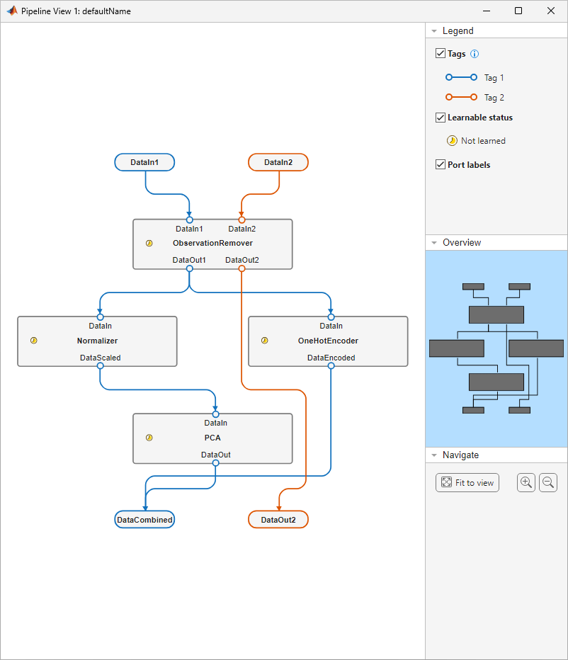
The pipeline accepts two input variables (DataIn1 and DataIn2) and returns two output variables (DataCombined and DataOut2). The first input variable (DataIn1) passes through the ObservationRemover component, then the Normalizer and OneHotEncoder components, and finally the PCA component. The second input variable (DataIn2) passes through the ObservationRemover component only.
Add Classification Component to Pipeline
Create a classificationSVMComponent object that trains a binary SVM classifier.
svmClassifier = classificationSVMComponent
svmClassifier =
  classificationSVMComponent with properties:

            Name: "ClassificationSVM"
          Inputs: ["Predictors"    "Response"]
       InputTags: [1 2]
         Outputs: ["Predictions"    "Scores"    "Loss"]
      OutputTags: [1 0 0]


Learnables (HasLearned = false)
    TrainedModel: []


Structural Parameters (locked)
      UseWeights: 0


Show all parameters
The component accepts two input variables (Predictors and Response) and returns three output variables (Predictions, Scores, and Loss). The component contains one learnable variable, TrainedModel, which is currently empty.
Add the classification component to the pipeline using the series object function. Then view the pipeline.
svmPipeline = series(pipeline,svmClassifier)
svmPipeline =
  LearningPipeline with properties:

             Name: "defaultName"
           Inputs: ["DataIn1"    "DataIn2"]
        InputTags: [1 2]
          Outputs: ["Predictions"    "Scores"    "Loss"    "DataOut2"]
       OutputTags: [1 0 0 2]

       Components: struct with 5 entries
      Connections: [12×2 table]

    HasLearnables: true
       HasLearned: false


Show summary of the components
view(svmPipeline)
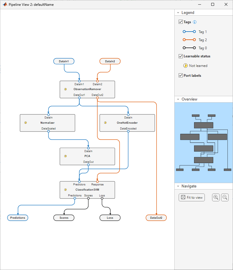
The pipeline accepts two input variables (DataIn1 and DataIn2) and returns four output variables (Predictions, Scores, Loss, and DataOut2). The first input variable (DataIn1) passes through the ObservationRemover component, Normalizer and OneHotEncoder components, PCA component, and ClassificationSVM component, in that order. The second input variable (DataIn2) passes through the ObservationRemover component, followed by the ClassificationSVM component.
Pass Data to Pipeline to Learn Parameters
Pass the car data to the classification pipeline svmPipeline by using the learn object function. The function uses the data to set the learnable parameter values in the Normalizer, OneHotEncoder, PCA, and ClassificationSVM components. Return the learned pipeline and the training loss value.
[learnedPipeline,~,~,learningLoss] = learn(svmPipeline,XTrain,YTrain)
learnedPipeline =
  LearningPipeline with properties:

             Name: "defaultName"
           Inputs: ["DataIn1"    "DataIn2"]
        InputTags: [1 2]
          Outputs: ["Predictions"    "Scores"    "Loss"    "DataOut2"]
       OutputTags: [1 0 0 2]

       Components: struct with 5 entries
      Connections: [12×2 table]

    HasLearnables: true
       HasLearned: true


Show summary of the components
learningLoss =
0.1703
View the pipeline with learned parameter values.
view(learnedPipeline)
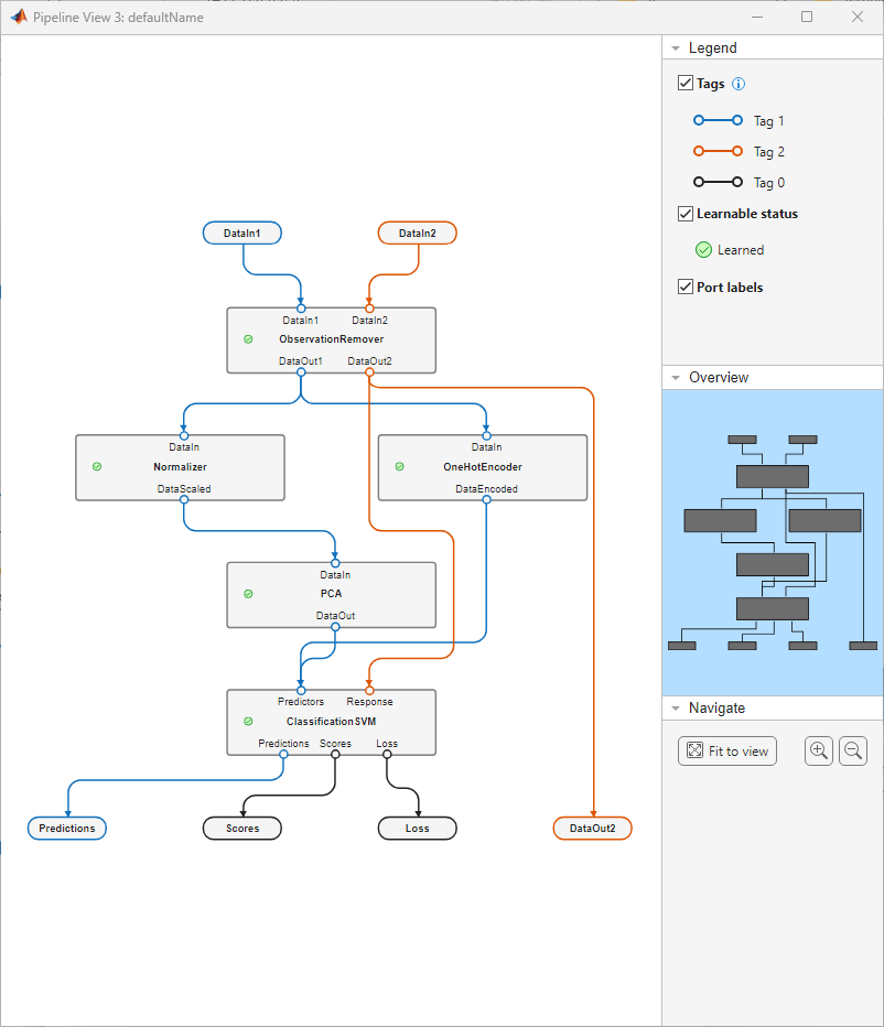
The pipeline view indicates that all the components have been learned. Note the green Learned icon in the Legend pane on the right under Learnable status. This same icon now appears in the components.
You can access the values of component learnables by using dot operation. For example, inspect the PCA coefficients computed by the PCA component and the SVM model trained by the ClassificationSVM component.
learnedPCACoefficients = learnedPipeline.Components.PCA.Coefficients
learnedPCACoefficients = 5×3

   -0.3311    0.8757    0.1481
    0.4831    0.1305    0.3849
    0.4845   -0.1304    0.1797
   -0.4460   -0.3087    0.8358
    0.4726    0.3224    0.3149
learnedSVMModel = learnedPipeline.Components.ClassificationSVM.TrainedModel
learnedSVMModel =
  CompactClassificationSVM
           PredictorNames: {1×16 cell}
             ResponseName: 'Origin'
    CategoricalPredictors: []
               ClassNames: [NotUSA    USA]
           ScoreTransform: 'none'
                    Alpha: [124×1 double]
                     Bias: 1.1291
         KernelParameters: [1×1 struct]
           SupportVectors: [124×16 double]
      SupportVectorLabels: [124×1 double]


  Properties, Methods
Evaluate Pipeline Performance
Pass the test data and the learned pipeline to the run function to see how the pipeline performs on new data.
[YPred,~,testingLoss] = run(learnedPipeline,XTest,YTest)
YPred=121×1 table
    predictions
    ___________

      USA
      USA
      USA
      USA
      USA
      USA
      USA
      USA
      USA
      NotUSA
      USA
      USA
      NotUSA
      USA
      USA
      USA
      ⋮
testingLoss =
0.1818
Create a confusion chart to visualize the correctly and incorrectly classified observations.
confusionchart(table2array(YTest),table2array(YPred))
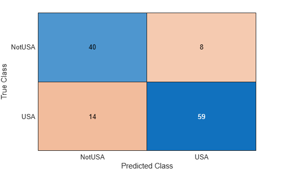
The test loss value is higher than the loss computed by learn, but this can be expected when you are classifying new data. The pipeline correctly classifies most of the observations, and the misclassification rate for each class is fairly even. You can try modifying pipeline component parameters to improve the classification accuracy, or use the learned model to classify unlabeled data.