Boundary Effects and the Cone of Influence
This topic explains the cone of influence (COI) and the convention Wavelet Toolbox™ uses to compute it. The topic also explains how to interpret the COI in the scalogram plot, and exactly how the COI is computed in cwtfilterbank and cwt.
Load the Kobe earthquake seismograph signal. Plot the scalogram of the Kobe earthquake seismograph signal. The data is sampled at 1 hertz.
load kobe
cwt(kobe,1)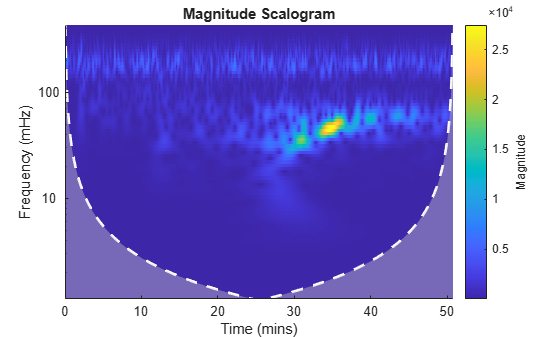
In addition to the scalogram, the plot also features a dashed white line and shaded gray regions from the edge of the white line to the time and frequency axes. Plot the same data using the sampling interval instead of sampling rate. Now the scalogram is displayed in periods instead of frequency.
cwt(kobe,seconds(1))
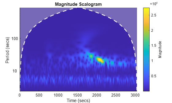
The orientation of the dashed white line has flipped upside down, but the line and the shaded regions are still present.
The white line marks what is known as the cone of influence. The cone of influence includes the line and the shaded region from the edge of the line to the frequency (or period) and time axes. The cone of influence shows areas in the scalogram potentially affected by edge-effect artifacts. These are effects in the scalogram that arise from areas where the stretched wavelets extend beyond the edges of the observation interval. Within the unshaded region delineated by the white line, you are sure that the information provided by the scalogram is an accurate time-frequency representation of the data. Outside the white line in the shaded region, information in the scalogram should be treated as suspect due to the potential for edge effects.
CWT of Centered Impulse
To begin to understand the cone of influence, create a centered impulse signal of length 1024 samples. Create a CWT filter bank using cwtfilterbank with default values. Use wt to return the CWT coefficients and frequencies of the impulse. For better visualization, normalize the CWT coefficients so that the maximum absolute value at each frequency (for each scale) is equal to 1.
x = zeros(1024,1);
x(512) = 1;
fb = cwtfilterbank;
[cfs,f] = wt(fb,x);
cfs = cfs./max(cfs,[],2);
Use the helper function helperPlotScalogram to the scalogram. The code for helperPlotFunction is at the end of this example. Mark the location of the impulse with a line.
ax = helperPlotScalogram(f,cfs);
hl = line(ax,[512 512],[min(f) max(f)], ...
    [max(abs(cfs(:))) max(abs(cfs(:)))]);
title("Scalogram of Centered Impulse")
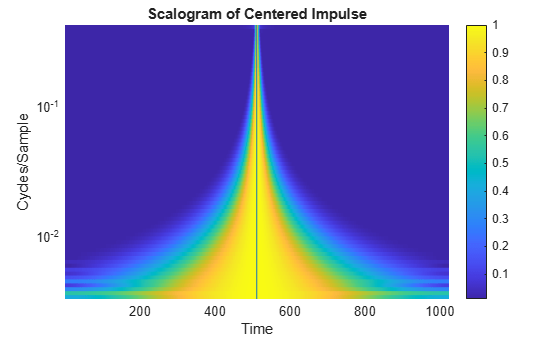
The solid black line shows the location of the impulse in time. Note that as the frequency decreases, the width of the CWT coefficients in time that are nonzero and centered on the impulse increases. Conversely, as the frequency increases, the width of the CWT coefficients that are nonzero decreases and becomes increasingly centered on the impulse. Low frequencies correspond to wavelets of longer scale, while higher frequencies correspond to wavelets of shorter scale. The effect of the impulse persists longer in time with longer wavelets. In other words, the longer the wavelet, the longer the duration of influence of the signal. For a wavelet centered at a certain point in time, stretching or shrinking the wavelet results in the wavelet "seeing" more or less of the signal. This is referred to as the wavelet's cone of influence.
Boundary Effects
The previous section illustrates the cone of influence for an impulse in the center of the observation, or data interval. But what happens when the wavelets are located near the beginning or end of the data? In the wavelet transform, we not only dilate the wavelet, but also translate it in time. Wavelets near the beginning or end of the data inevitably "see" data outside the observation interval. Various techniques are used to compensate for the fact that the wavelet coefficients near the beginning and end of the data are affected by the wavelets extending outside the boundary. The cwtfilterbank and cwt functions offer the option to treat the boundaries by reflecting the signal symmetrically or periodically extending it. However, regardless of which technique is used, you should exercise caution when interpreting wavelet coefficients near the boundaries because the wavelet coefficients are affected by values outside the extent of the signal under consideration. Further, the extent of the wavelet coefficients affected by data outside the observation interval depends on the scale (frequency). The longer the scale, the larger the cone of influence.
Repeat the impulse example, but place two impulses, one at the beginning of the data and one at the end. Also return the cone of influence. For better visualization, normalize the CWT coefficients so that the maximum absolute value at each frequency (for each scale) is equal to 1.
dirac = zeros(1024,1);
dirac([1 1024]) = 1;
[cfs,f,coi] = wt(fb,dirac);
cfs = cfs./max(cfs,[],2);
helperPlotScalogram(f,cfs)
title("Scalogram of Two-Impulse Signal")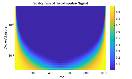
Here it is clear that the cone of influence for the extreme boundaries of the observation interval extends into the interval to a degree that depends on the scale of the wavelet. Therefore, wavelet coefficients well inside the observation interval can be affected by what data the wavelet sees at the boundaries of the signal, or even before the signal's actual boundaries if you extend the signal in some way.
In the previous figure, you should already see a striking similarity between the cone of influence returned by cwtfilterbank or plotted by the cwt function and areas where the scalogram coefficients for the two-impulse signal are nonzero.
While it is important to understand these boundary effects on the interpretation of wavelet coefficients, there is no mathematically precise rule to determine the extent of the cone of influence at each scale. Nobach et al. [2] define the extent of the cone of influence at each scale as the point where the wavelet transform magnitude decays to 2% of its peak value. Because many of the wavelets used in continuous wavelet analysis decay exponentially in time, Torrence and Compo [3] use the time constant to delineate the borders of the cone of influence at each scale. For Morse wavelets, Lilly [1] uses the concept of the "wavelet footprint," which is the time interval that encompasses approximately 95% of the wavelet's energy. Lilly delineates the COI by adding 1/2 the wavelet footprint to the beginning of the observation interval and subtracting 1/2 the footprint from the end of the interval at each scale.
The cwtfilterbank and cwt functions use an approximation to the rule to delineate the COI. The approximation involves adding one time-domain standard deviation at each scale to the beginning of the observation interval and subtracting one time-domain standard deviation at each scale from the end of the interval. Before we demonstrate this correspondence, add the computed COI to the previous plot.
helperPlotScalogram(f,cfs,coi)
title("Scalogram with Cone of Influence")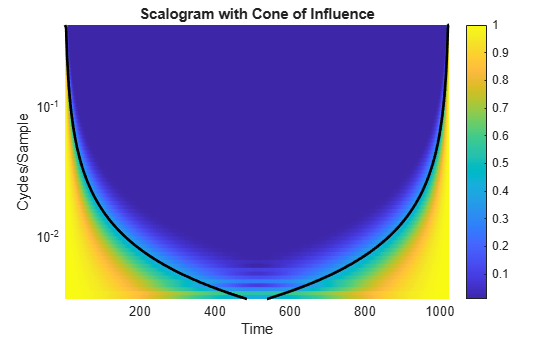
You see that the computed COI is a good approximation to boundaries of the significant effects of an impulse at the beginning and end of the signal.
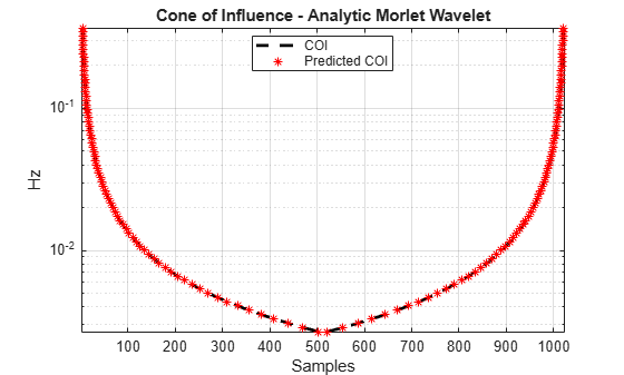
To show how cwtfilterbank and cwt compute this rule explicitly, consider two examples, one for the analytic Morlet wavelet and one for the default Morse wavelet. Begin with the analytic Morlet wavelet, where our one time-domain standard deviation rule agrees exactly with the expression of the folding time used by Torrence and Compo [3].
fb = cwtfilterbank(Wavelet="amor");
[~,f,coi] = wt(fb,dirac);
The expression for the COI in Torrence and Compo is , where is the scale. For the analytic Morlet wavelet in cwtfilterbank and cwt, this is given by:
cf = 6/(2*pi);
predtimes = sqrt(2)*cf./f;
Plot the COI returned by cwtfilterbank along with the expression used in Torrence and Compo.
plot(1:1024,coi,"k--",LineWidth=2)
hold on
grid on
plot(predtimes,f,"r*")
plot(1024-predtimes,f,"r*")
hold off
set(gca,YScale="log")
axis tight
legend("COI","Predicted COI",Location="best")
xlabel("Samples")
ylabel("Hz")
title("Cone of Influence - Analytic Morlet Wavelet")
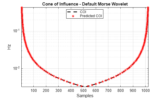
The last example shows the same correspondence for the default Morse wavelet in cwtfilterbank and cwt. The time-domain standard deviation of the default Morse wavelet is 5.5008, and the peak frequency is 0.2995 cycles/sample. Use the center frequencies of the wavelet bandpass filters as well as the time-domain standard deviation rule to obtain the predicted COI and compare against the values returned by cwtfilterbank.
fb = cwtfilterbank;
[~,f,coi] = wt(fb,dirac);
sd = 5.5008;
cf = 0.2995;
predtimes = cf./f*sd;
figure
plot(1:1024,coi,"k--",LineWidth=2)
hold on
grid on
plot(predtimes,f,"r*")
plot(1024-predtimes,f,"r*")
hold off
set(gca,'yscale',"log")
axis tight
legend("COI","Predicted COI",Location="best")
xlabel("Samples")
ylabel("Hz")
title("Cone of Influence - Default Morse Wavelet")
Appendix
The following helper function is used in this example.
helperPlotScalogram
function varargout = helperPlotScalogram(f,cfs,coi)
nargoutchk(0,1);
ax = newplot;
surf(ax,1:1024,f,abs(cfs),EdgeColor="none")
ax.YScale = "log";
clim([0.01 1])
colorbar
grid on
ax.YLim = [min(f) max(f)];
ax.XLim = [1 size(cfs,2)];
view(0,90)

xlabel("Time")
ylabel("Cycles/Sample")

if nargin == 3
    hl = line(ax,1:1024,coi,ones(1024,1));
    hl.Color = "k";
    hl.LineWidth = 2;
end

if nargout > 0
    varargout{1} = ax;
end

end
References
[1] Lilly, J. M. “Element analysis: a wavelet-based method for analysing time-localized events in noisy time series.” Proceedings of the Royal Society A. Volume 473: 20160776, 2017, pp. 1–28. dx.doi.org/10.1098/rspa.2016.0776.
[2] Nobach, H., Tropea, C., Cordier, L., Bonnet, J. P., Delville, J., Lewalle, J., Farge, M., Schneider, K., and R. J. Adrian. "Review of Some Fundamentals of Data Processing." Springer Handbook of Experimental Fluid Mechanics (C. Tropea, A. L. Yarin, and J. F. Foss, eds.). Berlin, Heidelberg: Springer, 2007, pp. 1337–1398.
[3] Torrence, C., and G. Compo. "A Practical Guide to Wavelet Analysis." Bulletin of the American Meteorological Society. Vol. 79, Number 1, 1998, pp. 61–78.
See Also
Apps
- Signal Analyzer (Signal Processing Toolbox)
Functions
cwt|cwtfilterbank|pspectrum(Signal Processing Toolbox)