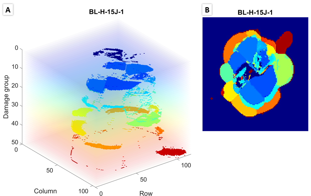
Processes C-scans, calculates time-of-flight, identifies contours of damaged regions, and creates a 3D reconstruction of the damage state
https://github.com/jessica-chan-5/ultrasonic-c-scan-segmentation-for-composites
You are now following this Submission
- You will see updates in your followed content feed
- You may receive emails, depending on your communication preferences
This code was developed as part of Jessica Chan’s master’s thesis in Dr Hyonny Kim’s lab at UC San Diego. The code takes pulse-echo ultrasonic C-scan data in character delimited formats (.csv, .txt, .dat) of aerospace composites with impact damage and creates a 3D reconstruction of the damage state. The code also calculates time-of-flight, creates a mask of the overall damaged region, and merges front and back C-scans of a sample when available. The code was developed in MATLAB 2022b, but works for 2019b or later.
Despite a high strength to weight ratio, aerospace composites are susceptible to impact damage which can be barely visible while still adversely affecting their strength, therefore detecting and characterizing damage is important. Non-destructive evaluation, specifically single-sided pulse-echo ultrasonic C-scans, can be used to detect damage. The main characteristic of barely visible impact damage is that it occurs from impacts that leave little to no visual indication on the front side that damage has occurred, when in fact there is internal damage, namely planar delaminations between the lamina, and there can be visual indication of damage on the back side of the component. Examples of barely visible impact damage include damage to a component impacted by runway debris, hail, or accidentally dropped maintenance tools 1.
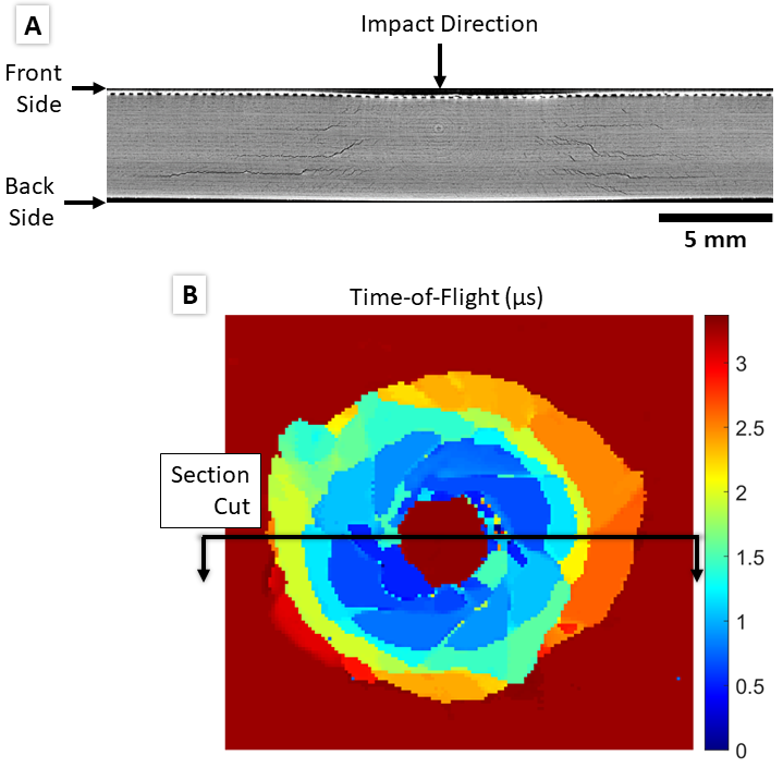
(A) Example through-thickness X-ray CT scan slice showing barely visible impact damage labeled with impact direction and front/back side with respect to impact direction. Reprinted with permission 2. (B) Processed UT C-scan of the same sample as in (A) showing front side damage and representative location for section cut shown in (A).
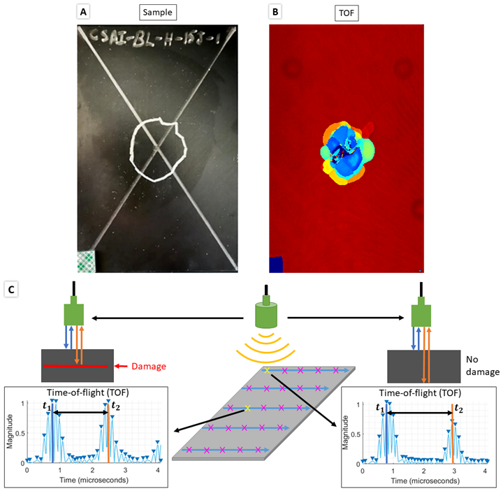
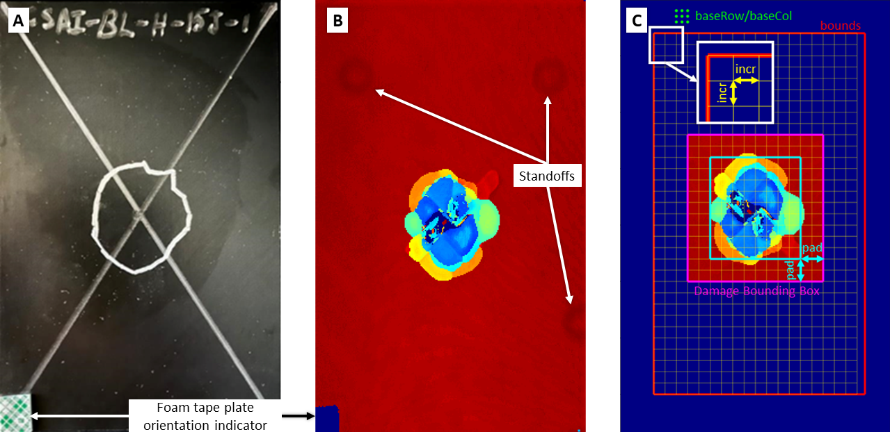
Pulse-echo UT C-scans are made of a 2D array of A-scans taken at points in a uniform grid across a sample. Each A-scan is the measurement of the reflection(s) from the initial ultrasonic signal emitted by the transducer. The first reflected peak is from the top layer of the sample and the second reflected peak is the topmost damaged interface within the sample. An example of the A-scan signal and time-of-flight (TOF) calculation for an undamaged and damaged A-scan point is shown in below. A map of the depth of damaged areas can be created by calculating the difference between the first peak and the second peak, the TOF, which then can be converted to damage depth by using the material’s through-thickness wave velocity.
(A) Photo of a sample with manually mapped damage region outline, (B) UT C-scan time-of-flight map, (C) C-scan process and calculating TOF for undamaged scan point (right) and damaged scan point (left) using the A-scan signal at each scan point.
-
UC San Diego Research Data Collection (RDCP): Code development and testing dataset along with processed output/figures are posted here with documentation about how the data was collected and created
-
Jessica Chan’s master’s thesis, Chapter 3: Code development is a detailed description of how the code functions
-
Barrett Romasko’s master’s thesis: Used 26 of 81 C-scans from this dataset collected by Barrett to develop and test the code (this is part of what is posted in the UC San Diego RDCP collection)
-
Mac Delany’s master’s thesis: Used front and back C-scan from sample LV-162 to validate code in conjunction with Andrew’s work on the same sample
-
Andrew Ellison’s PhD dissertation: Used CT X-ray scan and processed UT C-scan of the front side of LV-162 to validate code
-
Andrew Ellison’s shadow delamination paper: Paper presents a shadow extension algorithm demonstrated using the LV-162 sample for predicting shape of shadowed damaged regions which could be combined with this code in the future to create a more complete 3D reconstruction of the damage state
-
MathWorks File Exchange: Releases of the code are also published here, however, most updated version of code will always live on GitHub.
Thank you to:
- Professor Hyonny Kim for advising me on the development of this code
- Barrett Romasko for testing and scanning the composite sample dataset used for testing and development
- Andrew Ellison for explaining to me how to process C-scans and processing the C-scans and X-ray CT scan of the sample used to validate the code
- Mac Delany for testing and scanning the composite sample dataset used for validating the code
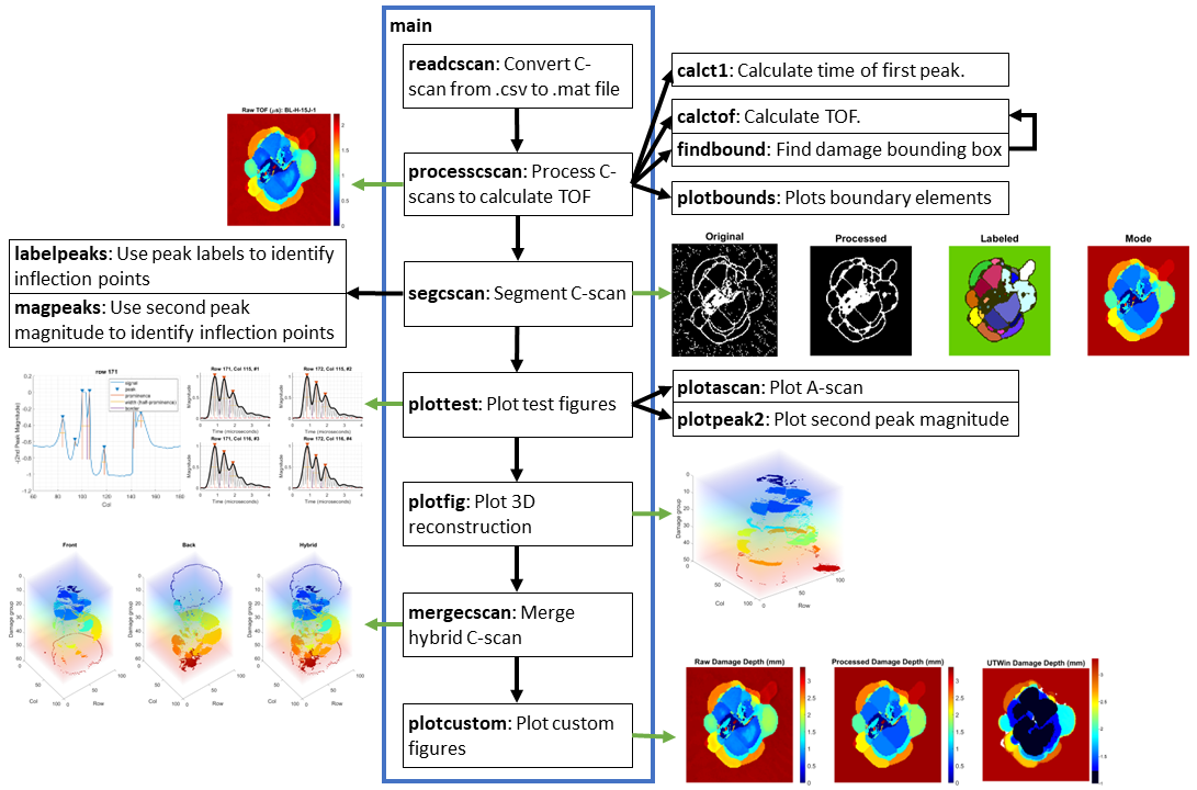
The overall structure of the code is shown below as a summary:
- Install the following MATLAB toolboxes if you don’t have them already:
- Curve Fitting Toolbox
- Image Processing Toolbox
- Parallel Computing Toolbox
- Signal Processing Toolbox
-
When running the code for the first time, it is suggested to test one sample first before attempting to process all samples in order to adjust parameters. Pick a sample you would like to use.
-
We will be using
test.mto adjust parameters, which is an exact copy ofmain.mbut with parallel for loops removed to allow for helper figures to appear. Parallel for loops do not allow for figures to appear. Parameters can be copied over after finishing adjusting. -
Just like MATLAB built in functions, type
help functionNameinto the Command Window for documentation
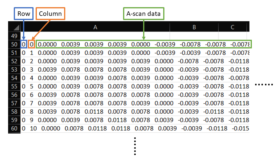
- Format your raw UT C-scan data in a supported character delimited file type (.csv, .txt, .dat) following the format below (header information is okay and will be trimmed automatically):
-
Run
foldersetup.min the same directory as the code to create the required folder structure for inputs, outputs, and figures. -
Move all formatted raw UT C-scan data into the Input folder
-
Open
test.mand edit Section ii to be a string array list of your file names. When adjusting parameters, you will only have one file name, but in general it will look like this:fileNames = ["sample-1";"sample-2","sample-3"];
If there is a sample with front and back side C-scans, fileNames should be formatted as the following:
fileNames = ["sample-1";"sample-1-back"];
-
In Section A, update
delimandfileExtto the character delimiter (i.e. ' ', ',') and file extension (including '.', i.e. '.csv') -
If your data does not have equal resolution along both dimensions, calculate the appropriate down sampling required to have equal resolution. Update
dRowanddColaccordingly. For example, if the data has equal resolution, leave both to 1. If you would like to sample every point along the row direction, setdRowto 1, but you would like to sample every 5th point along the column direction, setdColto 5. -
In
test.m, Section iii, edit all read function values to be false except forrunRead -
Run
test.mand go toOutput\cscanto check if the saved .mat files are the expected size. They should be size[row x column x data points per A-scan].
-
In
test.m, Section B, enter the sampling period,dt, in microseconds used to collect the A-scan signals -
First we will set the parameters for finding a rectangular box bounding the damaged region. The relevant parameters are illustrated below:
-
The purpose of
bounds, in red, is to define a search area that excludes artifacts that may be erroneously detected as damage such as the foam tape plate orientation indicator and standoffs the sample may be resting on. You can make an initial guess for an appropriate search area using the sampling resolution to convert to matrix indices. It should be in[startRow endRow startCol endCol]format in Section B. -
Choose a reasonable value for
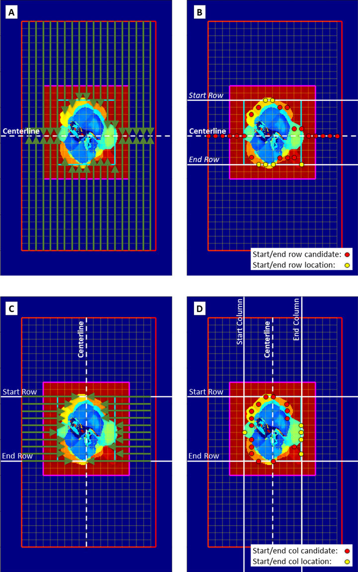
incr, this is in matrix indices and will define the coarse grid size, in yellow, used to search for the start of damage. The search method is shown below:
Damage bounding box search process. (A) Search along columns, (B) picking start row and end row indices, (C) search along rows, (D) picking start and end column indices.
-
Pick a grid of points using
baseRowandbaseColthat represent a grid of points in an undamaged region of the sample, shown as green dots. A baseline TOF will be calculated using the mode of these points -
Leave
pad,cropThresh,minProm1,noiseThresh,maxWidthat the orginal value, this will be adjusted later. -
If intersted in creating a dent depth map, set
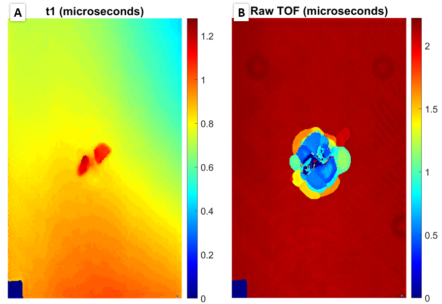
t1equal to true. This will increase run time significantly as it requires the whole sample to be processed. An example of a first peak TOF figure is shown below to the left with the raw TOF on the right for reference:
-
Set
resto the desired resolution for all saved figures in dpi (dots per inch). SetfontSizeto desired font size for all saved figures in pixels (same font size measurements as in Microsoft Word or Google Docs) -
In
test.m, Section iii, edit all read function values to be false except forrunProcessandtestProcessthen runtest.m -
Use the damage bounding box figure to adjust
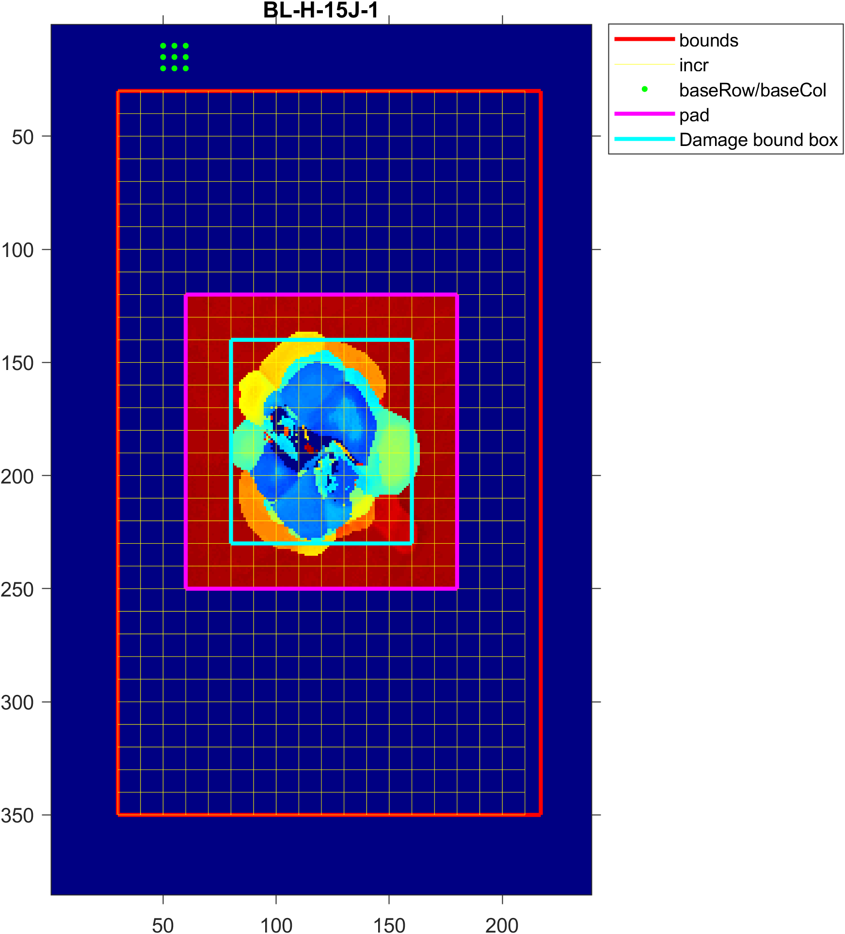
bounds,incr,baseRow,baseCol, andpadaccordingly. An example of the figure is shown below:
If regions of damage are being cropped by the damage bounding box, increase pad by the number of incr needed to expand the bounding box, in blue, to include the whole damage area. Decrease pad if desired to create a tighter bounding box. pad should be a whole number and is defined as (1 + pad x incr) added to all sides of the damage bounding box.
- Use the damage bounding box figure and queryable raw TOF figure to check if
cropThreshshould be increased or decreased by querying TOF values at relevant points. If the difference between the current grid search point and the calculated baseline TOF is greater thancropThresh, then the point is detected as damaged.
*Note: The helper figures produced by this code will be flipped about the x-axis (rows) because of MATLAB plotting idiosyncrasies, but the row, column and TOF values are correct.
-
Skip ahead to
plottest, it will be useful for adjustingminProm1,noiseThresh,maxWidthfromprocesscscan -
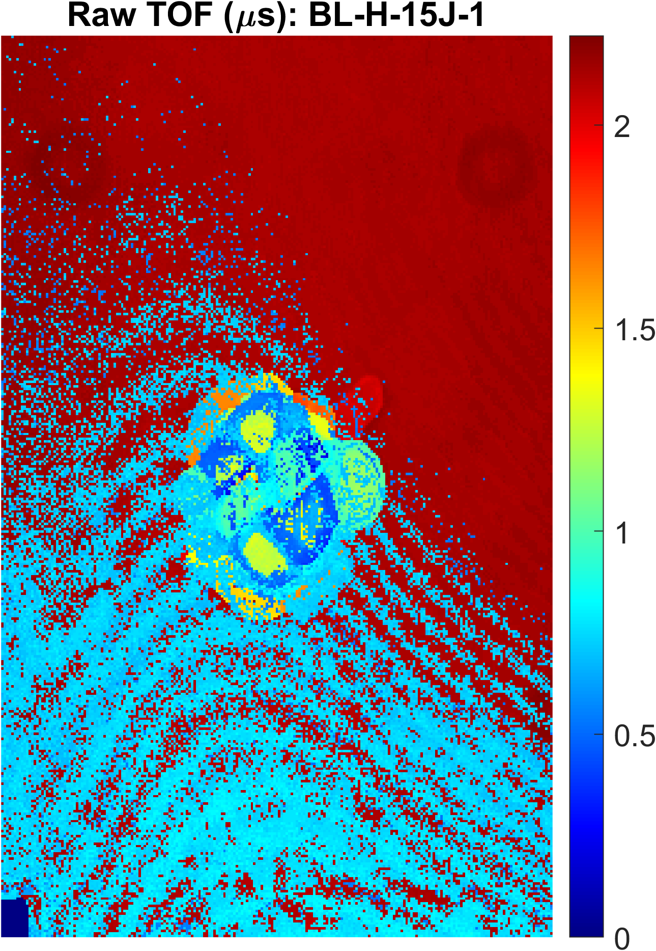
Shown below is a raw TOF figure showing the results of setting
minProm1too low (minProm1= 0):
-
Using the queryable raw TOF figure, query the row and column locations of a light blue artifact region. In
test.m, in Section D, setrowRangeandcolRangeto the rows and columns of interest. -
In Section iii, edit all read function values to be false except for
runTestthen runtest.m -
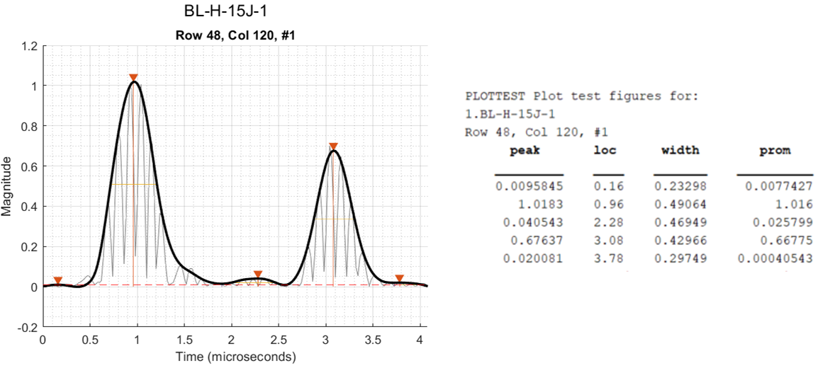
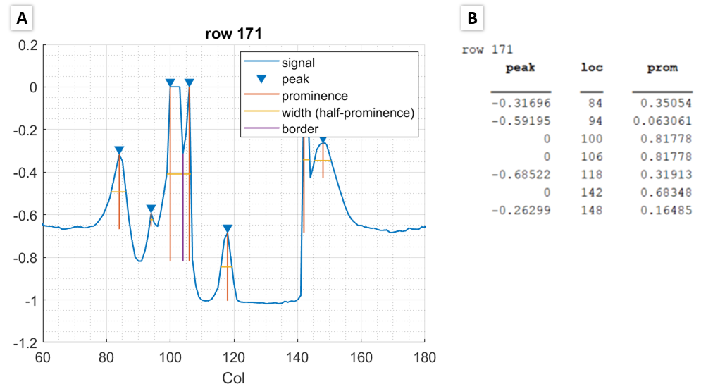
An example of the output is shown below with the figure and the Command Window output side-by-side:
In the above example, the first, third, and fifth peaks are a result of noise and slight changes in the data and do not represent peaks of interest. Prominence is a measure of how much a peak stands out because of its height and location relative to neighboring peaks. Any peaks with a prominence less than minProm1 is not detected. By looking at the corresponding prominence value printed in the Command Window, a good choice for minProm1 is 0.03, so that only the second and fourth peak are detected.
-
Steps 2-4 can be repeated, if necessary, for setting
noiseThresh. If the average of the signal at a point is less thannoiseThresh, the point is not processed and set to zero. -
Steps 2-4 can be repeated for setting
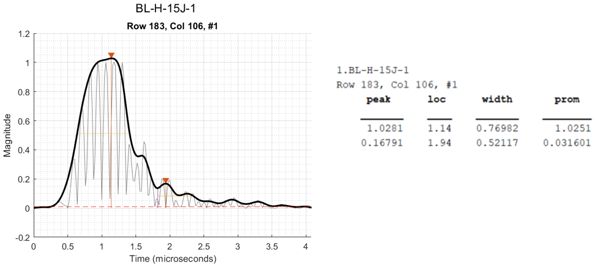
maxWidth. If the width of a peak is greater thanmaxWidth, then the peak is marked as "wide". These points are skipped when segmenting the TOF insegcscan. An example of a "wide" peak is shown below. These peaks represent damage that is close to the surface, blue, but where more than one peak is detected.
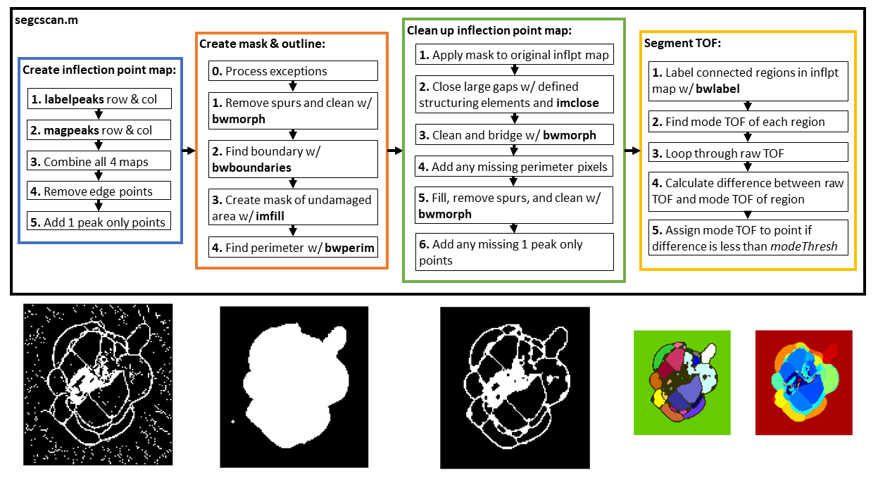
- An overview of how
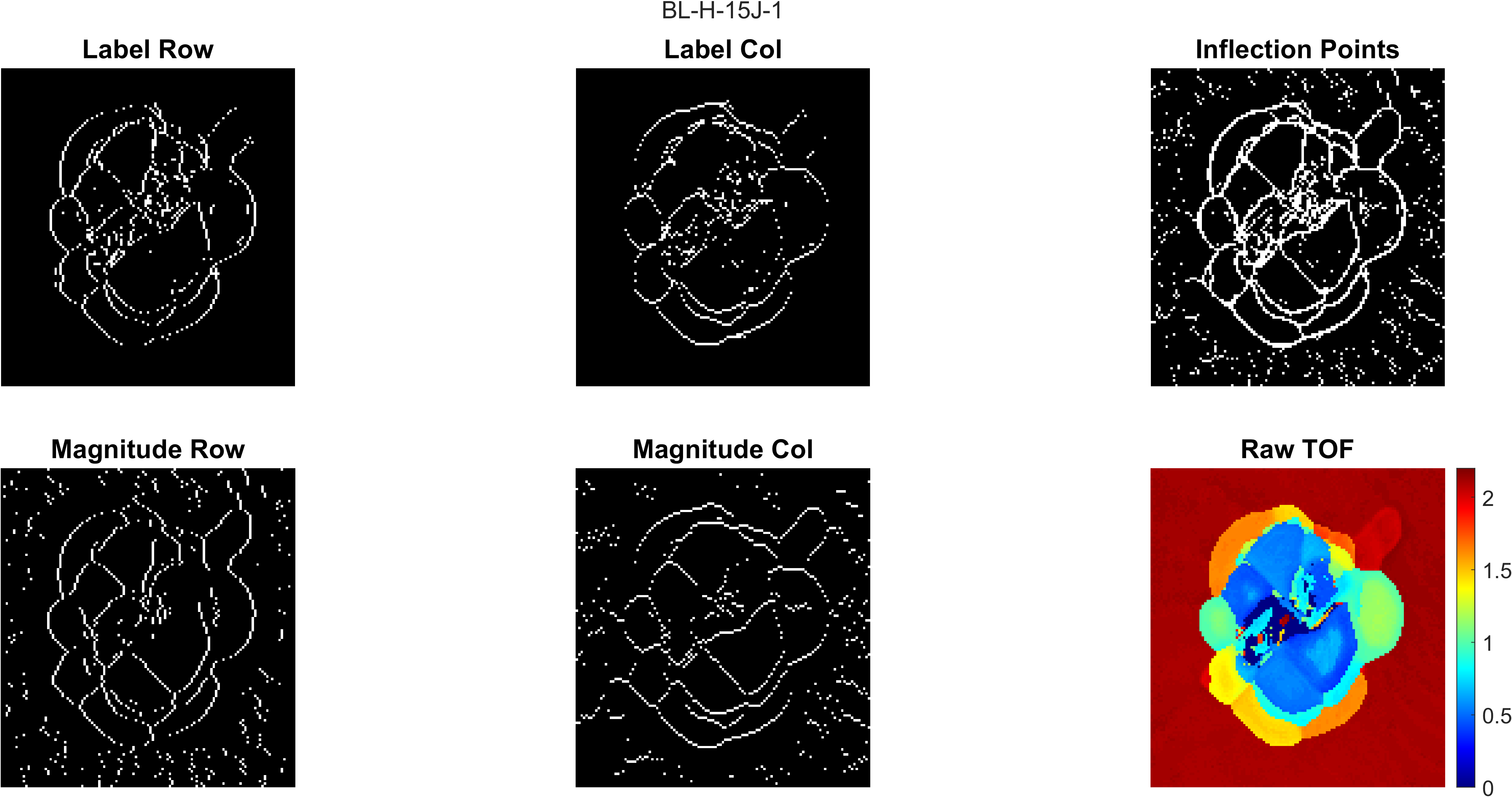
segcscanworks is shown below:
Inflection points in this code refer to points that outline where the damage changes from one layer to another in the laminate. labelpeaks and magpeaks process the raw TOF from processcscan row-wise and column-wise in order to obtain an inflection point map. All four resulting inflection point maps are combined using an OR operation. Morphological processing is used to clean up, close gaps, and label connected regions in the inflection point map. The TOF value in each labeled connected region is assigned to the mode value of the region it is a part of. For details of the process, see Section 3.6 of Jessica's MS thesis (Link to be included when published).
-
In
test.m, in Section C, leaveminProm2,peakThreshat original value. This will be adjusted later. -
Set
modeThreshtohigand seEl to[0 0 0 0] -
In Section iii, edit all read function values to be false except for
runSegandtestSegthen runtest.m -
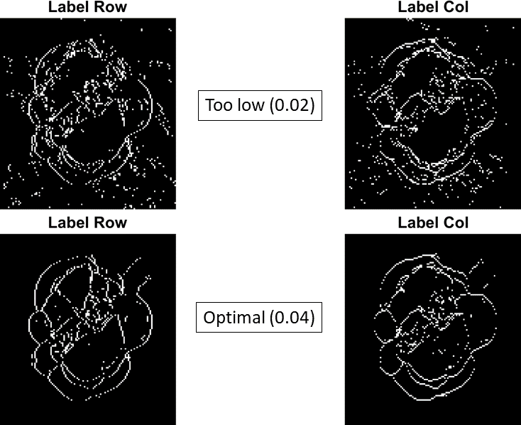
Adjust
peakThreshusing the combination inflection point figure. Below is an example ofpeakThreshset too low (peakThresh= 0.02) and an adjusted optimalpeakThreshvalue (peakThresh= 0.04):
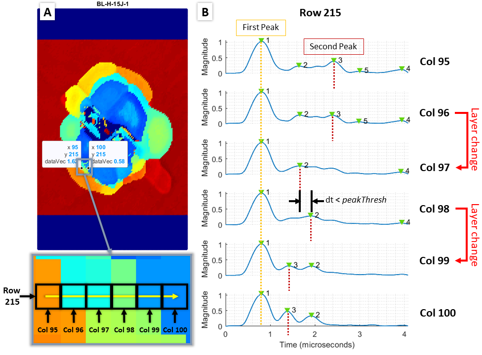
A figure explaining how peakThresh is used is shown below:
In the peak labeling process, each peak in each A-scan receives a unique numerical label. If a peak location change is greater than peakThresh, then the peak is considered a new unique peak and given a different label. Inflection points are marked when the second peak changes labels such as Column 96-97 and Column 98-99 in the example above. As mentioned in the summary of segcscan, the peak labeling and inflection point finding process occurs twice, once along rows and once along columns.
It is recommended to adjust peakThresh as a multiple of the sampling period, dt. In the example above the two different values of peakThresh were 1 x dt (0.02) and 2 x dt (0.04) respectively.
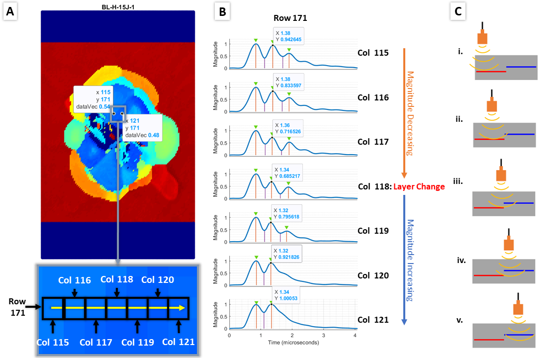
- Skip to
plottestagain. It will be used to help adjustminProm2. A figure explaining howminProm2is shown below:
minProm2 is used to exclude noisy peaks when looking at the magnitude of the second peak across a row or column. In this example, the layer change occurs at Column 118, where the magnitude of the second peak is at a local mininum.
*Note: in the plot of second peak magnitude, the negative value is taken to turn local mininum into local maximums so that the built-in MATLAB function findpeaks can detect them.
-
Pick a direction for
dir('row' or 'col') and a row or column number fornumin Section D. A good starting point is to look at the centerline along the row or column direction. -
In Section iii, edit all read function values to be false except for
runTestthen runtest.m -
Use the second peak magnitude figure and Command Window output to adjust
minProm2. An example is shown below:
- The combination inflection point figure from
segcscan, shown below, should also be used in tandem to adjust theminProm2value. A higherminProm2value will create a less noisy inflection points map, but with more gaps and a lowerminProm2value will create a noisier map, but with less gaps.
- Use the process and queryable inflection points figure to adjust
seElinput. TheseElinput is in[length45 length-45 length90 length0]format, where each value designates the length of the structuring element in pixels. The first value is a structuring element in the shape of a one pixel wide line angled at 45 degrees, with the rest in the same form. If there are gaps not filled by the default morphological processing steps in the code, then the user should use the least number of elements and the shortest elements necessary to close the gaps. The structuring elements are used to morphologically close the gaps. However, morphological closing can also connected undesired regions together.
For example, if there is a 4 pixel gap at 45 degrees, then a 5 pixel, 45 degree structuring element should be used. If values are left as zero, that structuring element is not used. The length should always be one pixel longer than the biggest gap present.
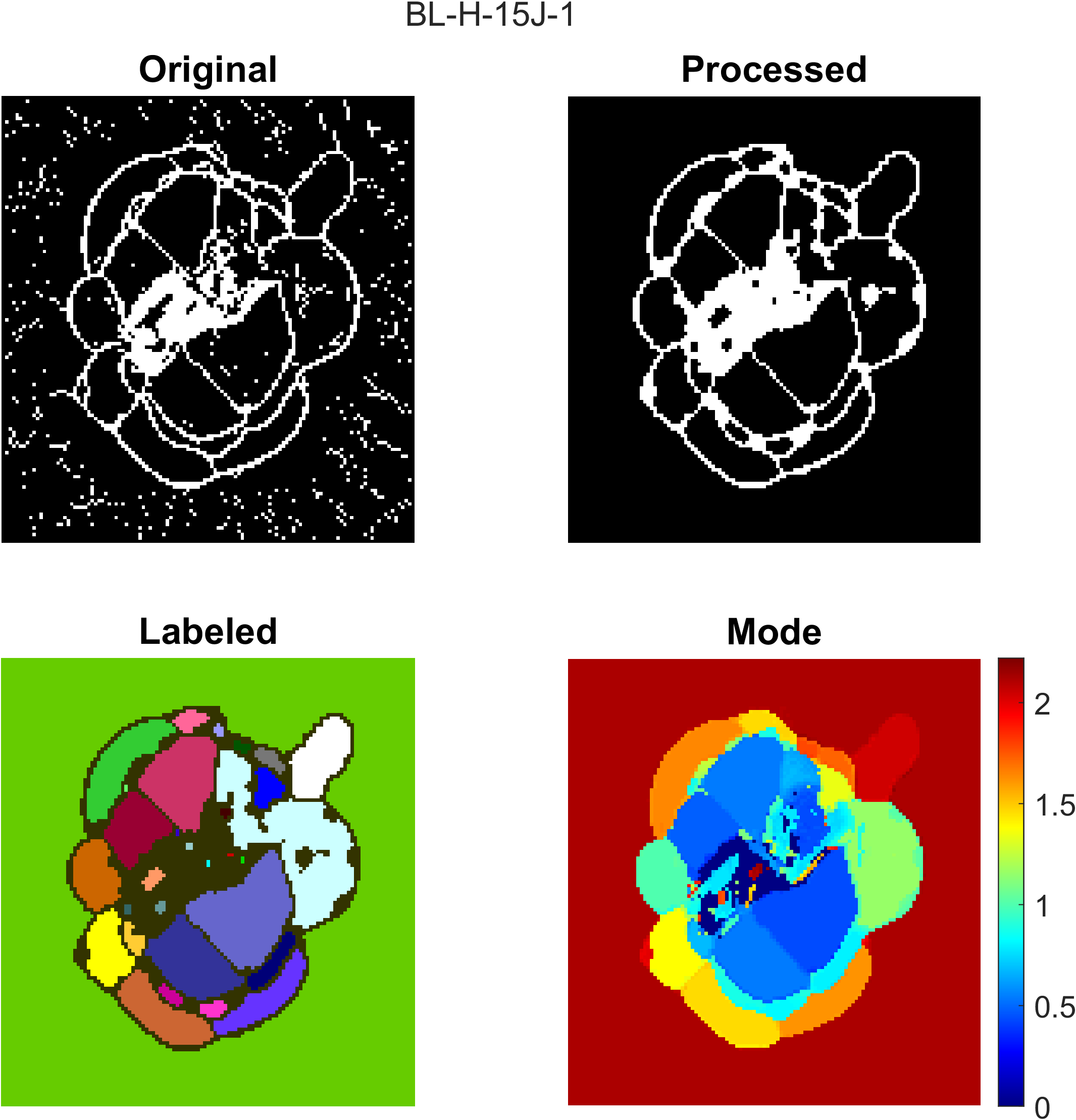
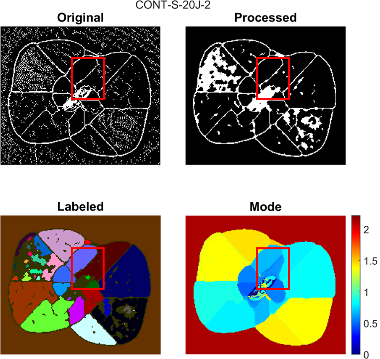
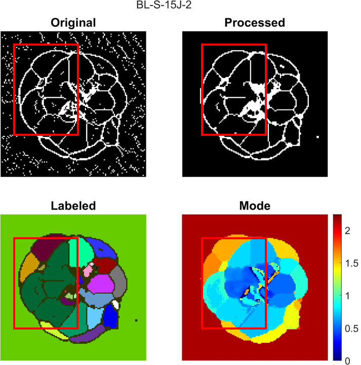
An example of the process figure is shown below, where the top right plot is the morphologically processed inflection points map and the bottom left plot is a plot of the labeled connected regions plotted by color. Each color represents an enclosed damaged region.
- Use the process, compare, queryable raw TOF and queryable inflection points figure to adjust the
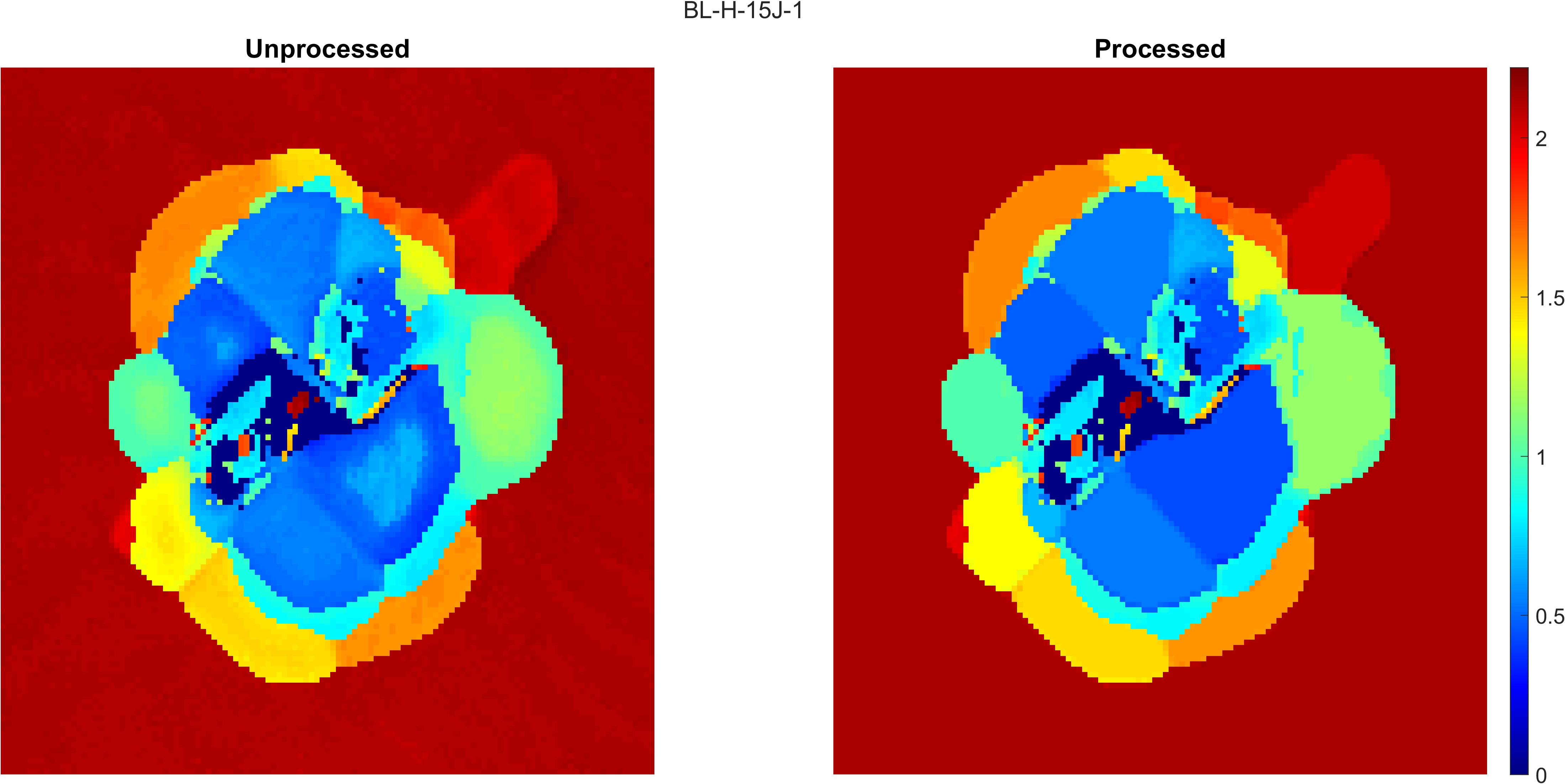
modeThreshinput. This input can be used for gradually transitioning regions that are not currently detectable by the code or near surface damage that is also currently unable to be detected. Examples of near surface damage requiring lowermodeThreshinput is shown below.
modeThresh is used to process the TOF map. If the difference between the TOF value of the current point and the mode value of the connected region it belongs to is greater than modeThresh, then the TOF value at the point is not changed to the mode value of the connected region. Additionally, the boundaries of the connected regions are not included in any connected regions, so all TOF values located at a boundary are not changed.
A lower modeThresh value means that the processed TOF map will look more similar to the raw TOF map and that less artifacts will be removed. A higher modeThresh value means that the processed TOF map will have more artifacts removed, but gradual changes in TOF value or close to surface damage regions may merge together.
Suggested modeThresh values of hig, med, and low are included in the test.m file in Section C.
A compare figure is shown below as an example of where more artifacts are removed:
-
Update
plateThickto the thickness of your sample in mm andnLayersto the number of layers in the sample layup. -
In Section iii, edit all read function values to be false except for
runFigthen runtest.m -
Check damage layer figures in 2D and 3D to see if results are as expected. Examples are shown below:
-
This section is only applicable if there are front and back side C-scans of sample(s).
-
In Section iii, edit
filesMergeto be 1. When processing more than one sample with front and back C-scans, the file indices included should be front C-scans only. So iffileNamewas:
fileName = ["sample-1","sample-2","sample-1-back","sample-2-back"]
Then, filesMerge should be:
filesMerge = 1:2
Adjust the file index offset, di, if there is a mix of front side C-scans only samples and front/back side C-scan samples. For example, if fileName was:
fileName = ["sample-1","sample-2","sample-3","sample-4","sample-3-back","sample-4-back"]
Then di should be equal to 2 (index of first front/back scan - 1).
-
Set
dxanddyMergeCscanfor each sample to be equal to zero. -
In Section iii, edit all read function values to be false except for
runMergeandtestMergethen runtest.m -
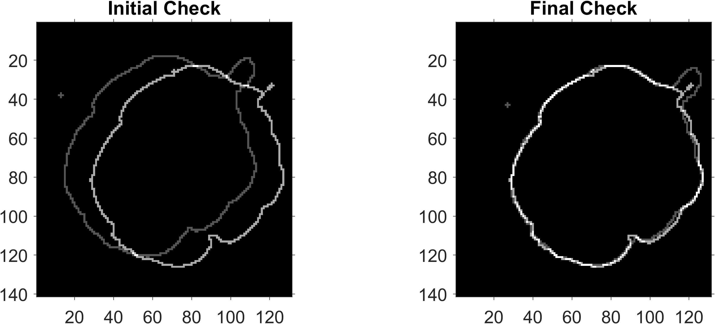
Use the merge check figure to adjust the front side C-scan damage outline vertically and horizontally relative to the back side C-scan.
Units are in pixels. dx left is negative, right is positive. dyMergeCscan down is negative, right is positive. The darker grey outline is the front outline and the lighter grey outline is the back outline.
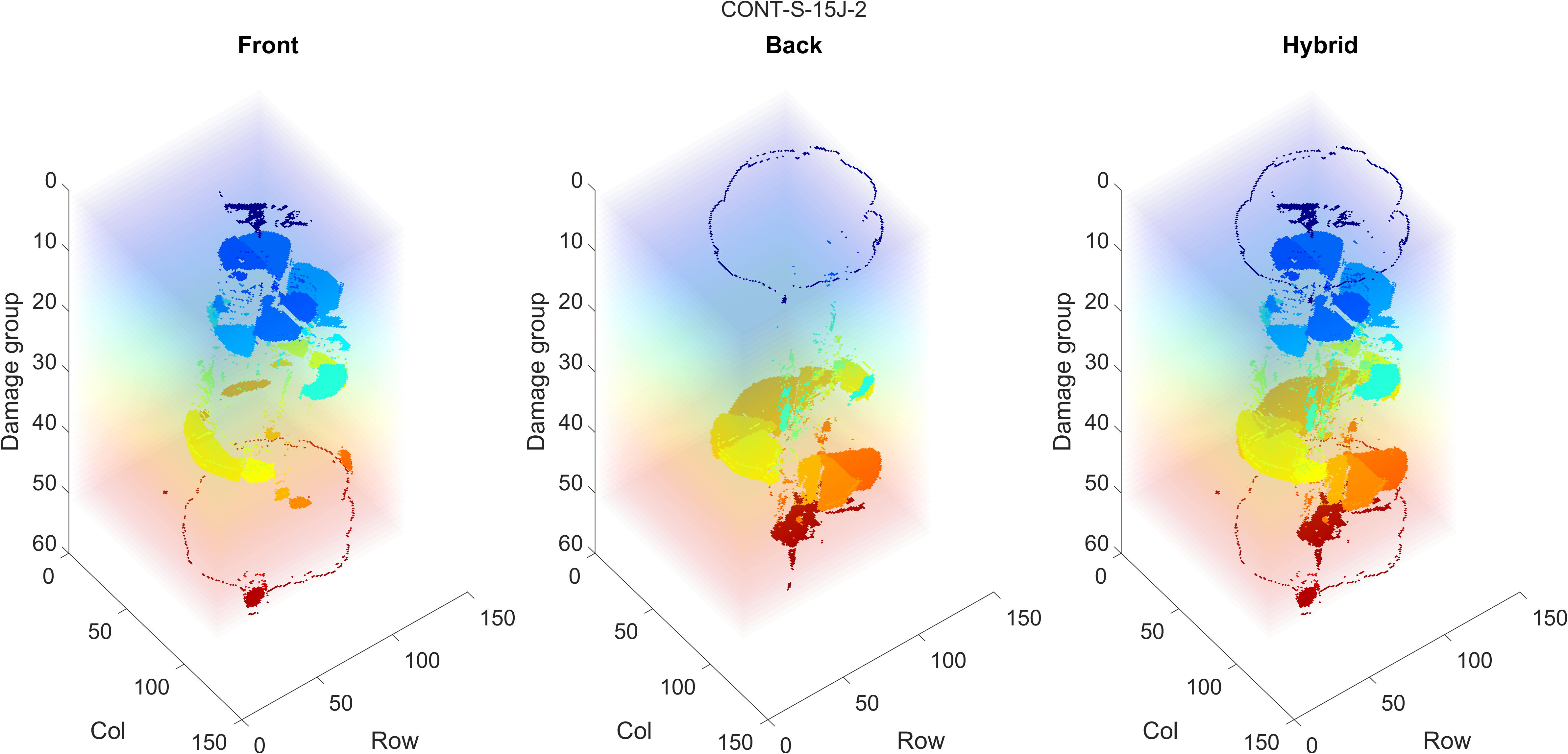
- When the outlines match up, check the front, back and hybrid 3D reconstruction figure. An example is shown below:
- This section may not be of interest to everyone, but can be adapted to plot other figures. The original purpose was to plot the unprocessed damage layer map, the processed damage layer map, and the Mistras/UTWin damage layer map side by side for comparison.
This function was kept in the code in case others want to plot comparisons with commercial C-scan processing sofware
-
Set
startRowUT,endRowUT,startColUT,endColUTto pixel row/col values to crop the UTWin screenshots to only include the damage layer map. GIMP or similar software can be used to find the appropriate crop values. -
In Section iii, edit all read function values to be false except for
runCustomandtestCustomthen runtest.m -
Similar to
mergecscan, updatedyPlotCustomto adjust the UTWin image vertically where up is positive and down is negative. -
Check the UTWin comparison figure to see if all damage maps are vertically aligned. An example is shown below:
As shown in the figure, the code is able to define lobes of damage near the surface that appear as dark blue and black in the UTWin image, which the sofware is unable to resolve. The processed damage map removes donut artifacts while retaining detail in the lobes near the top surface of the sample.
readcscan(fileName,inFolder,outFolder,delim,dRow,dCol)

   Requirement: Down sample to equal resolution along row and col

   Input: \inFolder\fileName.csv
   Output: \outFolder\fileName-
                               cscan.mat 3D matrix - [row x col x # data pts/A-scan]
processcscan(fileName,outFolder,figFolder,dt,bounds,incr,baseRow,baseCol,cropThresh,pad,minProm1,noiseThresh,maxWidth,calcT1,test,fontSize,res)

   Input: \outFolder\fileName-cscan.mat
   Output: \outFolder\fileName-
                               rawTOF   .mat 2D matrix – [row x col]
                               peak     .mat 2D matrix – [row x col]
                               locs     .mat 2D matrix – [row x col]
                               wide     .mat 2D matrix – [row x col]
                               nPeaks   .mat 2D matrix – [row x col]
                               cropCoord.mat 2D matrix – [1 x 4]
                               t1       .mat 2D matrix – [row x col]
   Figures: \figFolder\fileName-
                                t1.        .fig/.png
                                damBoundBox.fig/.png
                                rawTOFquery.fig
                                rawTOF     .fig/.png
   Functions:
      - calct1
      - calctof
      - findbound
      - implot
      - imsave
      - imscatter
      - plotbounds
segcscan(fileName,outFolder,figFolder,minProm2,peakThresh,modeThresh,seEl,test,fontSize,res)
   Input: \outFolder\fileName-
                               rawTOF   .mat 2D matrix – [row x col]
                               peak     .mat 2D matrix – [row x col]
                               locs     .mat 2D matrix – [row x col]
                               wide     .mat 2D matrix – [row x col]
                               nPeaks   .mat 2D matrix – [row x col]
                               cropCoord.mat 2D matrix – [1 x 4]
   Output: \outFolder\fileName-
                               tof   .mat 2D matrix – [row x col]
                               inflpt.mat 2D matrix – [cropRow x cropCol]
                               mask  .mat 2D matrix – [cropRow x cropCol]
                               bound .mat 2D matrix – [cropRow x cropCol]
                               peak2 .mat 2D matrix – [cropRow x cropCol]
   Figures: \figFolder\fileName-
                                comboInflpt         .fig/.png
                                inflptQuery         .fig
                                masks               .fig/.png
                                process             .fig/.png
                                compare             .fig/.png
                                tof                 .fig/.png
   Functions:
      - implot
      - imsave
      - imscatter
      - labelpeaks
      - magpeaks
plotfig (fileName,outFolder,figFolder,plateThick,nLayers,fontSize,res)
   Input: \outFolder\fileName-
                               tof      .mat 2D matrix – [row x col]
                               cropCoord.mat 2D matrix – [1 x 4]
                               mask     .mat 2D matrix – [cropRow x cropCol]
   Output: \outFolder\fileName-
                               damLayers.mat 2D matrix – [row x col]
   Figures: \figFolder\fileName-
                                damLayers.fig/.png
                                3Dplot   .fig/.png
   Functions:
      - implot
      - imsave
mergecscan (fileName,outFolder,figFolder,dx,dy,test,fontSize,res)

   Requirement: Same front and back C-scan dimensions [row x col]

   Input: \outFolder\fileName-
                               mask     .mat 2D matrix – [cropRow x cropCol]
                               damLayers.mat 2D matrix – [row x col]
                               cropCoord.mat 2D matrix – [1 x 4]
                               bound    .mat 2D matrix – [cropRow x cropCol]
   Output: \outFolder\fileName-
                               hybridCscan.mat 2D matrix – [cropRow x cropCol]
   Figures: \figFolder\fileName-
                                hybridCscan    .fig/.png
                                frontBackHybrid.fig/.png
   Functions:
      - imsave
plotcustom (fileName,inFolder,outFolder,figFolder,utwincrop,dy,plateThick,test,fontSize,res)
   Input:   \outFolder\fileName-
                                 rawTOF   .mat 2D matrix – [row x col]
                                 tof      .mat 2D matrix – [row x col]
                                 cropCoord.mat 2D matrix – [1 x 4]
            \inFolder\utwin\fileName      .bmp image file
   Figures: \figFolder\fileName-
                                 utwin    .fig/.png
   Functions:
      - implot
      - imsave
Footnotes
-
Federal Aviation Administration, "Advisory Circular: Composite Aircraft Structure," U.S. Department of Transportation, 2009. ↩
-
A. Ellison, "Segmentation of X-ray CT and Ultrasonic Scans of Impacted Composite Structures for Damage State Interpretation and Model Generation," PhD Dissertation, UC San Diego, 2020. ↩
Cite As
Jessica Chan (2026). Ultrasonic C-scan Segmentation for Composites (https://github.com/jessica-chan-5/ultrasonic-c-scan-segmentation-for-composites/releases/tag/v1.0.3), GitHub. Retrieved .
General Information
- Version 1.0.3 (5.37 MB)
-
View License on GitHub
MATLAB Release Compatibility
- Compatible with any release
Platform Compatibility
- Windows
- macOS
- Linux
| Version | Published | Release Notes | Action |
|---|---|---|---|
| 1.0.3 | See release notes for this release on GitHub: https://github.com/jessica-chan-5/ultrasonic-c-scan-segmentation-for-composites/releases/tag/v1.0.3 |
||
| 1.0.2.0 | See release notes for this release on GitHub: https://github.com/jessica-chan-5/ultrasonic-c-scan-segmentation-for-composites/releases/tag/v1.0.2 |
||
| 1.0.1 | See release notes for this release on GitHub: https://github.com/jessica-chan-5/ultrasonic-c-scan-segmentation-for-composites/releases/tag/v1.0.1 |
||
| 1.0.0 |


