2D Porous Flow Chemistry

Version 0.1.0 (7.71 MB) by Lyra Ladshaw

This is a repository for porous flow models using Matlab's PDE Toolbox. See the GitHub page for full set of equations from the README.

https://github.com/aladshaw3/porous_flow_matlab

0.0

(0)

43 Downloads

Updated 21 Aug 2023

View License on GitHub

Porous Flow in MATLAB

This repository provides a MATLAB interface for solving 2D PDEs resulting from reactive water flow through a porous media. The physics include:

Pressure driven advective/convective flow
Thermal balance of the fluid phase
Mass balance for chemicals in the fluid phase

Requirements

MATLAB
PDE Toolbox

Equation Set

Pressure driven Darcy flow

Thermal energy balance

<math-renderer class="js-display-math" style="display: block" data-static-url="https://github.githubassets.com/static" data-run-id="29e7de77f3b2ed2e7d273a4b946bfd5d">$$ (\varepsilon \rho c_{pw} + (1- \varepsilon) \rho_{s} c_{ps}) \frac{\partial T}{\partial t} - \nabla{ ( (\varepsilon K_w + (1- \varepsilon) K_s ) \cdot \nabla{T} ) } = - (\varepsilon \rho c_{pw}) \vec{v} \cdot \nabla{T} + \varepsilon \sum{\Delta H_j \cdot r_j } $$</math-renderer>

Mass balances (for each species)

<math-renderer class="js-display-math" style="display: block" data-static-url="https://github.githubassets.com/static" data-run-id="29e7de77f3b2ed2e7d273a4b946bfd5d">$$ \varepsilon \frac{\partial C_i}{\partial t} - \nabla{ ( \delta_i \varepsilon D_i \cdot \nabla{C_i} ) } = - \delta_i \varepsilon \vec{v} \cdot \nabla{C_i} + \varepsilon \sum{u_j \cdot r_j }$$</math-renderer>

Reaction term

Mobility term

If species is mobile...

Otherwise...

Other tools

This repo also contains a generalized set of utilies for creating gifs.

gif.m (Edited from the Original by Chad Greene)
create_gif.m (Creates gifs from a set of user defined commands)

These were used to create the example results shown below. See the tests directory for example usage.

Examples

All examples discussed have their source code under the tests directory.

(1) Basic Usage

Test file tests/test_porous_flow_2D_01.m contains some basic calculation checks for material properties, but also exercises the simulation tools basic use cases. The test case involves a simple square domain (4m x 4m) and a single chemical species with 2 first-order loss reactions.

Creating an instance

This example starts by initiallizing the porous_flow_2D object with vector spaces for 1 species, 2 reactions, and a single subdomain.

obj = porous_flow_2D(1, 2, 1);

Importing geometry for meshing

The geometry is created using the built in Matlab decsg function, however, you can import any geometry file to use. Once you have a defined geometry, you pass it into the porous_flow_2D object. You can also define the GeometryOrder and Hmax (i.e., maximum element size). The Matlab PDE toolbox will automatically generate the mesh from this information.

obj.set_geometry_from_edges(g, "quadratic", 0.25);

Editable material properties

Next, we can setup the information and parameters for the chemical species and reactions (as well as other properties such as particle size, bulk densities, thermal properties, etc.). A full listing of these properties can be found by reading through the porous_flow_2D object itself, but are also listed below.

    %% Public properties
    properties (Access = public)
        particle_diameter     % particle diameter in m
        particle_porosity     % Volume of micro-voids per bulk solids volume
        muA                   % Viscosity pre-exponential in kg/m/s
        muB                   % Viscosity temperature relation B in K
        muC                   % Viscosity temperature relation C in K 
        rhoA                  % Density temperature relation A in K^-2
        rhoB                  % Density temperature relation B in K^-1
        rhoC                  % Density temperature relation C in -
        rhoRef                % Reference Density in kg/m^3
        bulk_porosity         % system bulk porosity (vol voids / vol bulk solids)
        KozenyCarmannConst    % Kozeny-Carmann coefficient (dimensionless)
        diff_factor           % Diffusivity factor 
        alpha                 % Dispersion length factor in m
        refDiff               % Reference diffusivity in m^2/s
        refDiffTemp           % Reference diffusivity temperature in K
        cpA                   % Specific heat temperature parameter in K^-2
        cpB                   % Specific heat temperature parameter in K^-1
        cpC                   % Specific heat reference parameter -
        KwA                   % Thermal conductivity of water slope in K^-1
        KwB                   % Thermal conductivity of water intercept -
        char_len              % A characteristic length for the domain in m
        bulk_solids_dens      % Bulk solids density in the domain in kg/m^3
        bulk_solids_Cp        % Bulk solids heat capacity in J/kg/K
        bulk_solids_cond      % Bulk solids thermal conductivity in J/m/K/s

        mobile_spec_idx       % Matrix of 1s and 0s (where 1 indicates the species is mobile)
        rxn_stoich            % Stoichiometry matrix
        rxn_powers            % Matrix for reaction power terms
        rxn_rate_const        % Matrix for reaction rate constants (units will vary)
        rxn_act_energy        % Matrix for reaction rate activation energies (J/mol)
        rxn_enthalpy          % Matrix for reaction enthalpies (J/mol)

        model                 % PDE model object 

        boundaries            % Object to identify boundaries 
    end

Setting up FEM coefficient matrices

This Matlab object utilizes the General PDE toolbox system in Matlab. This system uses a faily complex, but comprehensive way to setup the matrix system for all variables in your system simultaneously. More details can be found in the links below:

To simplify this process, after you have finished editing any of the material properties from porous_flow_2D object, you can simply call the set_coefficients function to automatically have all these coefficient matrices built automatically.

NOTE: You will want to do this BEFORE applying Boundary Conditions (BCs)

obj.set_coefficients();

Setting up Boundary Conditions

Just like the coefficient matrices, the Matlab toolbox has a relatively complex set of subroutines for applying BCs. To simplify this, the porous_flow_2D object will automatically apply all the proper BCs for your problem based on whether it is an "input" or "output" boundary.

Input Boundary

To set the input boundaries, you need to supply:

The set of boundary ids
A fluid velocity at each id
An input temperature at each id
An input concentration for each species at each id (NxID)

inbound_set = [3,4];
velocity_set = [0.005,0.0075];
temperature_set = [298,298];
concentration_matrix = [1,0.5];
obj.set_input_boundaries(inbound_set, velocity_set, ...
                    temperature_set, concentration_matrix);

Output Boundary

To set the output boundaries, you only need to supply:

The set of boundary ids
Reference state pressure at the output boundaries

outbound_set = [1];
pressure_set = [101350];
obj.set_output_boundaries(outbound_set, pressure_set);

NOTE: Any boundary ID where you DO NOT specify boundary conditions will utilize the so-called "Natural BC" for a FEM problem, which is equivalent to a Neumann-type BC where the slope of the variable at the bounary is zero.

Setting up Initial Conditions

To set initial conditions (ICs), you need to provide values for each of the variables within each subdomain of the solution space. In this example, we only have 1 subdomain, so we just provide the variable ICs for pressure, temperature, and the 1 chemical species.

subdomain_set = [1];
pressure_set = [101350];
temperature_set = [298];
concentration_matrix = [0];
obj.set_initial_conditions(subdomain_set,pressure_set,temperature_set, concentration_matrix);

Setting up the time span and solving

To solve the system, simply create a t_span for the number of time steps and time positions to solve for, then call the solve_system function. At output, you will recieve "results" as a TimeDependentResults object. From this object, you can extract things such as the "NodalSolution" for post-processing and generating plots.

nsteps=20;
t_span = linspace(0,200,nsteps);
results = obj.solve_system(t_span);
u = results.NodalSolution;

Example 1 - Results

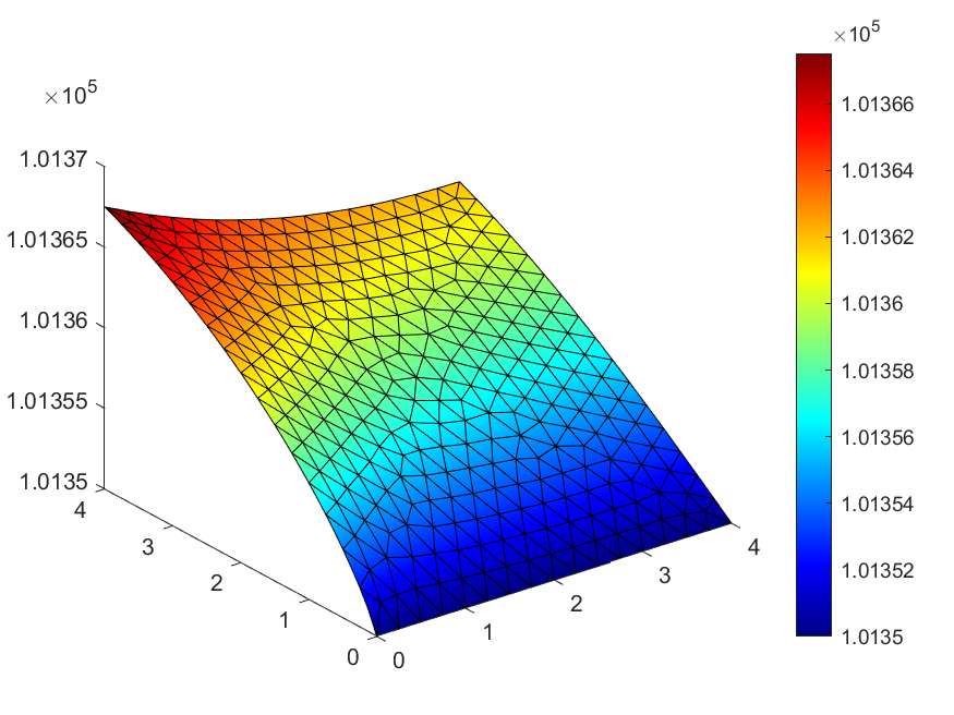
Figure 1: Pressure distribution (Pa)

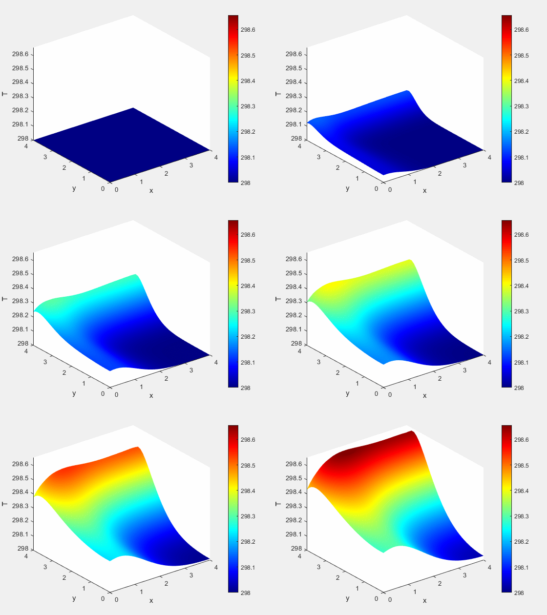
Figure 2: Temperature dynamics (K)

Figure 3: Concentration dynamics (mol/m^3)

(2) Injection well and Draw well

This example is meant to showcase some of the more interesting types of porous flow simulations, as well as the utilization of "immobile", which can be used to represent the formation of either precipitates or the adsorption process. It involves 2 species, 2 reactions, on 1 domain

% Create instance of PDE object 
%     2 chemical species, 2 reactions, 1 subdomain
obj = porous_flow_2D(2, 2, 1);

Pressure distribution from injection and water extraction

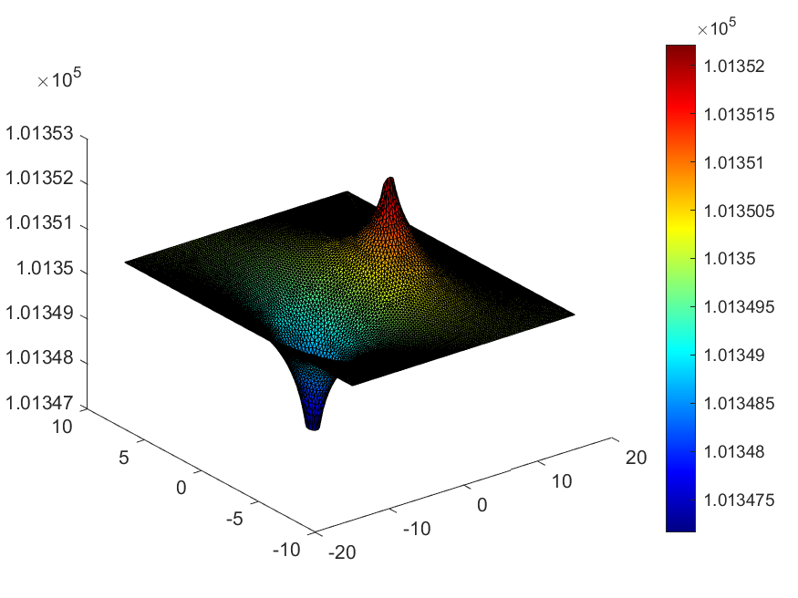
In this example, we have a rectangular domain from x = (-15, 15) meters and from y = (-10, 10) meters. Then, located at point (5,0) there is an injection well where warm saline water is being added. Not too far way, located at point (-5,0) there is a well that is extracting water at the same rate that the saline water is being injected at. This causes a high pressure zone at (5,0) and a low pressure zone at (-5,0).

Figure 4: Pressure distribution from wells (Pa)

How the Input Boundaries are setup to facilitate the pressure distribution

The high-pressure zone is where fluid is being added, thus it has a positive velocity. The low-pressure zone is where fluid is being removed, thus is has a negative velocity. These velocities are always orthogonal to the boundaries, so eventhough the boundaries are pointing in all directions, we only need to provide these "relative" velocities' at each boundary.

% Setup input BCs
%       5,6,7,8 - Injection of stuff
%       9,10,11,12 - Pulling water out
inbound_set = [5,6,7,8, 9,10,11,12];
velocity_set = [0.005,0.005,0.005,0.0005, -0.005,-0.005,-0.005,-0.005];
temperature_set = [315,315,315,315, 298,298,298,298];
concentration_matrix = [0.6,0.6,0.6,0.6, 0.0,0.0,0.0,0.0;
                        0.0,0.0,0.0,0.0, 0.0,0.0,0.0,0.0]; %NxID matrix of concentrations (2x8)
obj.set_input_boundaries(inbound_set, velocity_set, ...
                    temperature_set, concentration_matrix);

Defining a chemical species as "immobile"

There is a mobile_spec_idx property that can be used to denote a particular chemical species as "immobile" (by default, all species are assumed mobile). Lack of mobility of the 2nd species in this simulation is defined as:

obj.mobile_spec_idx(2,1,1) = 0; % 2nd species is immobile

NOTE: The 1st index is the species ID, the 2nd index is ALWAY 1 (needed for matrix structure), and the 3rd index is the subdomain ID.

Defining chemical reactions

By default, the system assumes that there are no reactions or that any reactions there are have a rate of 0, thus no impact. To add in reactions, we just need to modify the reaction information parameters:

% Set up reaction parameters
%       Triple indexs are (species id, rxn id, subdomain id)
%       Double indexs are (rxn id, subdomain id)

% Reaction 1:  A --> B   (where A id = 1, B id = 2)
%       r1 = k1*exp(-E1/R/T)*CA^1
obj.rxn_stoich(1,1,1) = -1; % negative means this species is consumed in this reaction
obj.rxn_stoich(1,2,1) = 1; %  positive means this species is formed in this reaction
obj.rxn_act_energy(1,1) = 25000; % activation energy for reaction 1
obj.rxn_rate_const(1,1) = 1e2; % Rate const
obj.rxn_powers(1,1,1) = 1; % si parameter from reaction term (power of A)
obj.rxn_enthalpy(1,1) = -0.5e6; % Negative enthalpy (this reaction generates heat)

% Reaction 2: B --> A
%       r2 = k2*exp(-E2/R/T)*CB^1
obj.rxn_stoich(2,1,1) = 1; % positive means this species is consumed in this reaction
obj.rxn_stoich(2,2,1) = -1; % negative means this species is formed in this reaction
obj.rxn_act_energy(2,1) = 55000; % activation energy for reaction 2
obj.rxn_rate_const(2,1) = 1e-2; % Rate const
obj.rxn_powers(2,2,1) = 1; % si parameter from reaction term (power of B)
obj.rxn_enthalpy(2,1) = 0.5e7; % Positive enthalpy (this reaction consumes heat)

Example 2 - Results

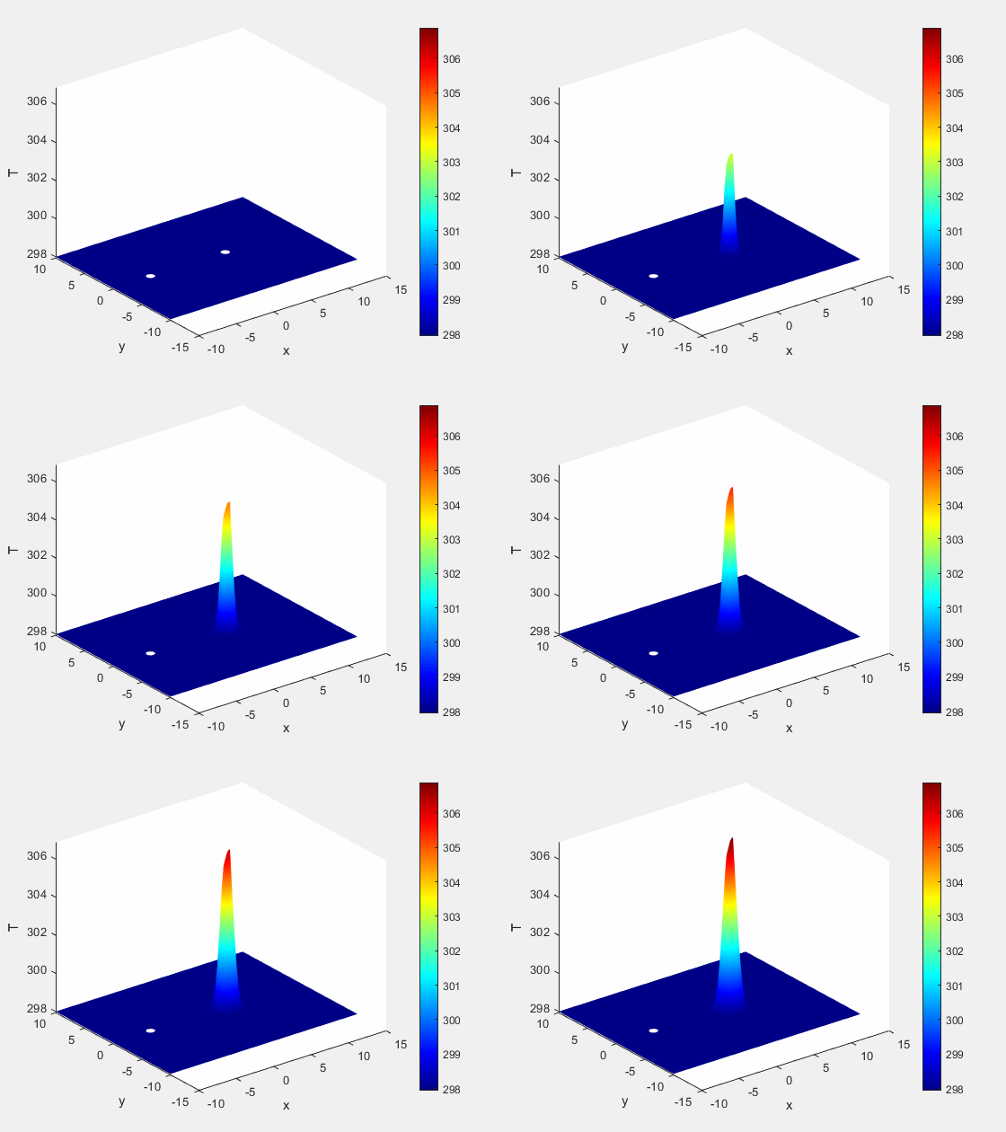
The simulation shows that as we inject this warm saline solution into the first well, that the water immediately adjacent to the injection well begins to heat.

Figure 5: Temperature dynamics (K)

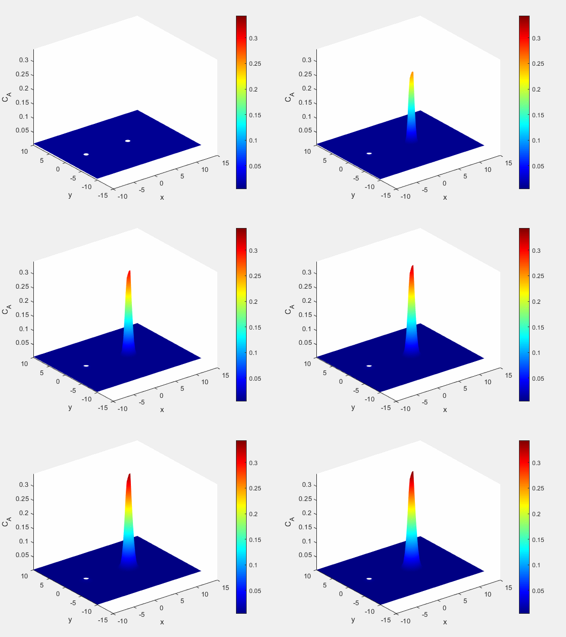
At the same time we see an increase in the salt content of the water immediately adjacent to the well, as well as the formation of some of our immobile species. This formation of immobile species also limits the distribution of the saline solution further from the point of injection.

Figure 6: Concentration of mobile saline species A (mol/m^3)

(3) Multi-domain Properties and Chemical Breakthrough

This last example was used to demonstrate how you can setup material properties and parameters in a system that has multiple subdomains with different properties. It also demonstrates how to create different types of plots to look at things like chemical breakthrough or distribution of chemicals across a domain.

Problem setup

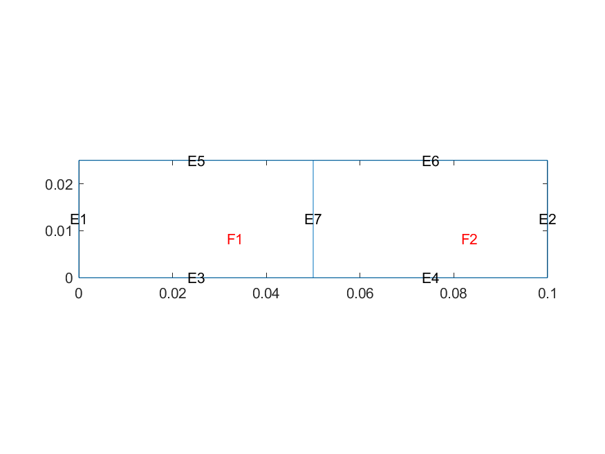
In this example, we will have a simple rectangular domain, but that full domain is composed of to different "Faces" that will represent 2 subdomains, each with different material properties.

Figure 7: Image of the subdomains

Distribution of properties and reactions

In this example, not only are the material properties different with subdomain, but also our set of reactions will be different in each subdomain. This is actually fairly common in catalysis applications for engineered chemical treatment systems.

% Create instance of PDE object 
%     4 chemical species, 4 reactions, 2 subdomains
obj = porous_flow_2D(4, 4, 2);

% Set geometry based on edges and setup functions
obj.set_geometry_from_edges(g,"linear",0.005);

% Set up reaction parameters: r1 --> A & B in Sub01
obj.rxn_stoich(1,1,1) = -1; %species id, rxn id, subdomain id
obj.rxn_act_energy(1,1) = 25000; % rxn id, subdomain id
obj.rxn_rate_const(1,1) = 1e3;
obj.rxn_powers(1,1,1) = 1;
obj.rxn_enthalpy(1,1) = -5e7;
obj.rxn_stoich(2,1,1) = 1; %species id, rxn id, subdomain id

% Set up reaction parameters: r2 --> B & C in Sub01
obj.rxn_stoich(2,2,1) = -1; %species id, rxn id, subdomain id
obj.rxn_act_energy(2,1) = 55000; % rxn id, subdomain id
obj.rxn_rate_const(2,1) = 1e8;
obj.rxn_powers(2,2,1) = 1;
obj.rxn_enthalpy(2,1) = 3e3;
obj.rxn_stoich(3,2,1) = 1; %species id, rxn id, subdomain id

% Set up reaction parameters: r3 --> C & D in Sub02
obj.rxn_stoich(3,3,2) = -1; %species id, rxn id, subdomain id
obj.rxn_act_energy(3,2) = 15000; % rxn id, subdomain id
obj.rxn_rate_const(3,2) = 5e1;
obj.rxn_powers(3,3,2) = 1;
obj.rxn_enthalpy(3,2) = 2e7;
obj.rxn_stoich(4,3,2) = 1; %species id, rxn id, subdomain id

% Set up reaction parameters: r4 --> D & C in Sub02
obj.rxn_stoich(4,4,2) = -1; %species id, rxn id, subdomain id
obj.rxn_act_energy(4,2) = 75000; % rxn id, subdomain id
obj.rxn_rate_const(4,2) = 1e3;
obj.rxn_powers(4,4,2) = 1;
obj.rxn_enthalpy(4,2) = -5e3;
obj.rxn_stoich(3,4,2) = 1; %species id, rxn id, subdomain id

obj.mobile_spec_idx(2,1,1) = 0; % B species is immobile in sub01
obj.mobile_spec_idx(2,1,2) = 0; % B species is immobile in sub02
obj.mobile_spec_idx(4,1,1) = 0; % D species is immobile in sub01
obj.mobile_spec_idx(4,1,2) = 0; % D species is immobile in sub02


% Setup subdomain physical constants
%       The 3rd index is the subdomain index
obj.bulk_porosity(1,1,1) = 0.33;
obj.bulk_porosity(1,1,2) = 0.45;
obj.particle_diameter(1,1,1) = 4e-3;
obj.particle_diameter(1,1,2) = 6e-3;
obj.char_len = obj.particle_diameter;
obj.bulk_solids_dens(1,1,1) = 2100;
obj.bulk_solids_dens(1,1,2) = 2500;
obj.bulk_solids_Cp(1,1,1) = 1.715e3;
obj.bulk_solids_Cp(1,1,2) = 1.115e3;


% Call this before setting BCs, but after setting parameters
obj.set_coefficients();

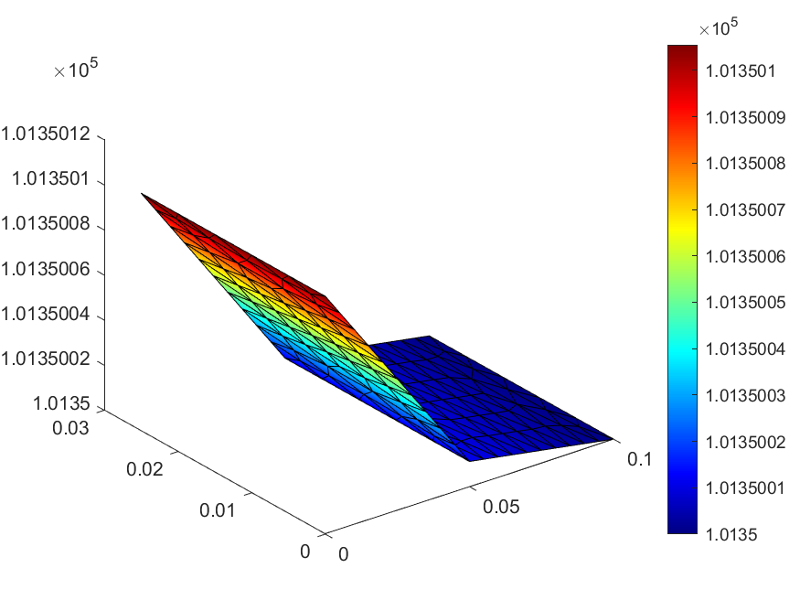
This distribution of physical parameters has a big impact on the pressure distribution in the system (see below).

Figure 8: Pressure distribution (Pa)

The first subdomain undergoes much higher pressure drop because it is composed of much smaller particles and has much less void space. Thus, it is necessary to apply more pressure here to get the same fluid flow rate as in the second domain.

Setting ICs for each subdomain

We will call the same ICs function from before, but this time we need to set the initial conditions for each subdomain. In this example, we set the same initial conditions regardless of subdomain, but you can use this same function call to set different ICs for each subdomain.

% Set initial conditions (for each subdomain)
subdomain_set = [1,2];
pressure_set = [101350,101350];
temperature_set = [298,298];
concentration_matrix = [0.0, 0.0;
                        0.0, 0.0;
                        0.0, 0.0;
                        0.0, 0.0];  % NxID (4x2)
obj.set_initial_conditions(subdomain_set,pressure_set,temperature_set, concentration_matrix);

Example 3 - Results

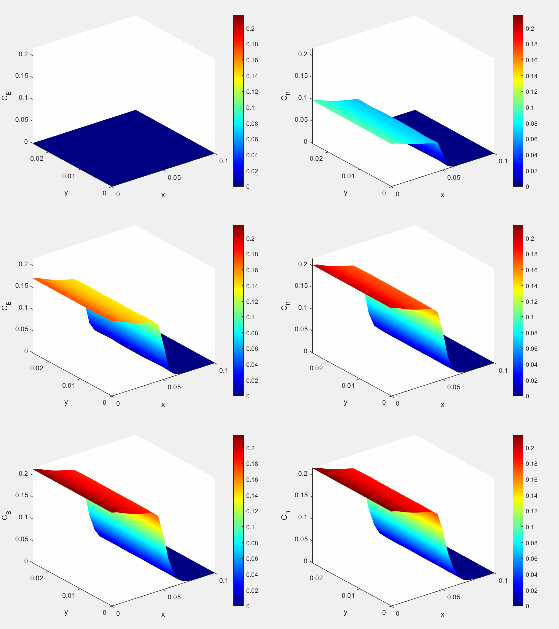
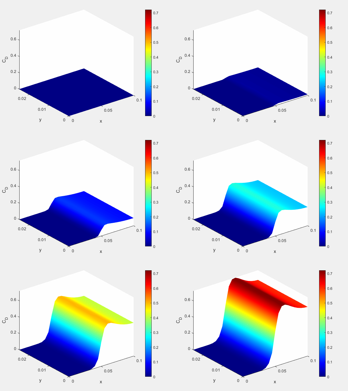
Because species B and D are immobile, and formed in different domains, we see that they will generally not be found in the other domain. However, since this is a FEM, there is some "diffusion" of these species between subdomains. This could be thought of as a "surface diffusion" between subdomains.

Figure 9: Concentration of immobile species B (mol/m^3)

Figure 10: Concentration of immobile species D (mol/m^3)

NOTE: This minor amount of "surface diffusion" is unavoidable in the Matlab PDE toolbox because we cannot fully "isolate" variables from a given subdomain in the Matlab toolbox.

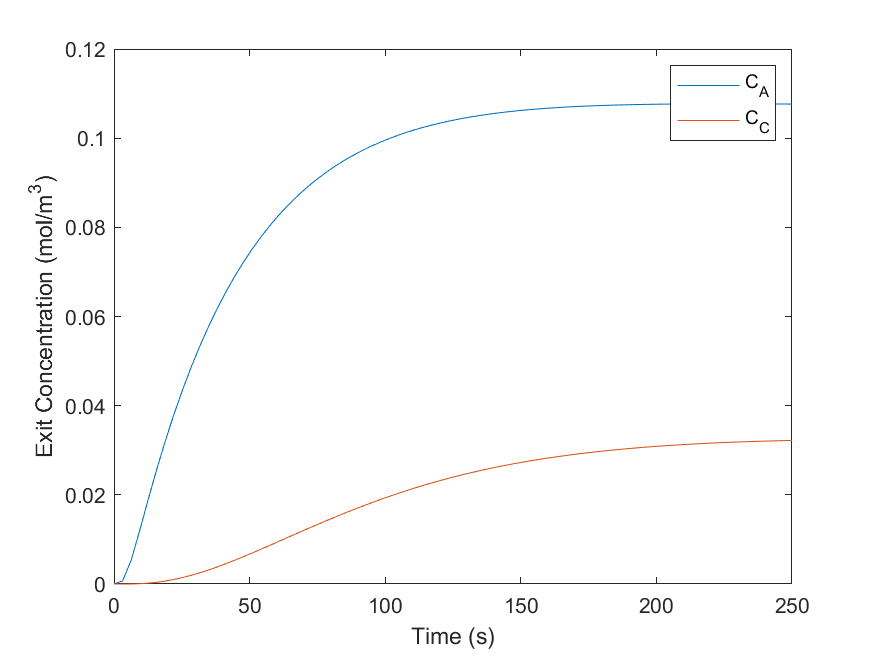
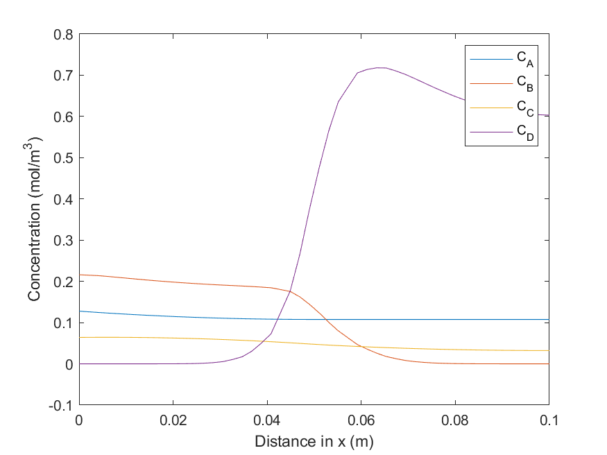
We can use the NodalSolution on output of the simulation, along with the interpolateSolution function in Matlab to generate plots for:

Breakthrough of mobile species at exit overtime

Figure 11: Concentrations of A and C at the exit of the domain overtime

Concentration distribution of all chemicals along simulation axis

Figure 12: Concentrations of all species along x-axis at end of simulation

NOTE: For source code examples and further explanation, see files under tests folder.

Citation

Ladshaw, A.P., "Porous Flow MATLAB: A simple 2D interface for modeling flow and reactions through porous media," https://github.com/aladshaw3/porous_flow_matlab, Accessed (Month) (Day), (Year).

Cite As

Lyra Ladshaw (2024). 2D Porous Flow Chemistry (https://github.com/aladshaw3/porous_flow_matlab/releases/tag/v0.1.0), GitHub. Retrieved July 27, 2024.

MATLAB Release Compatibility

Created with R2023a

Compatible with any release

Platform Compatibility

Windows macOS Linux

Tags Add Tags

Community Treasure Hunt

Find the treasures in MATLAB Central and discover how the community can help you!

Start Hunting!

load_directories.m

source

tests

Version	Published	Release Notes
0.1.0	21 Aug 2023		Download

To view or report issues in this GitHub add-on, visit the GitHub Repository.