coneplot
Plot cones in 3-D vector field
Syntax
Description
coneplot(
plots cones at sample locations (X,Y,Z,U,V,W,Cx,Cy,Cz)Cx, Cy,
Cz) within a Cartesian vector field. The magnitudes and orientations of
the cones are determined by the vector coordinates (X,
Y, Z) and the vector components
(U, V, W). The vector coordinates
define the location of each vector in 3-D space, and the vector components define the
magnitude and orientation of each vector.
coneplot(___, specifies a scale
factor for the lengths of the cones:s)
If
sis a positive number,coneplotadjusts the lengths of the cones so they do not overlap. Then it stretches the cones by a factor ofs. A scale factor of2doubles the lengths of the cones, and a scale factor of0.5halves the lengths of the cones. Larger values ofsmight result in overlapping cones.If
sis0,coneplotdoes not adjust or scale the lengths of the cones.
Specify s as the last argument in any of the preceding
syntaxes.
coneplot(___, specifies an
array for controlling the colors of the cones. The colors)colors array must be
the same size as one of the vector field arrays (X, Y,
Z, U, V, or
W).
coneplot(___,"quiver") draws arrows instead of cones.
This syntax does not support the colors argument.
coneplot(___, specifies the
interpolation method for calculating the magnitudes and orientations of the cones.method)
coneplot( plots into the
target axes ax,___)ax.
p = coneplot(___)Patch or Quiver object p.
Most syntaxes return a Patch object, but if you specify the
"quiver" option, coneplot returns a
Quiver object. Use p to set properties of the
object after creating it. For a list of properties, see Patch Properties or Quiver Properties.
Examples
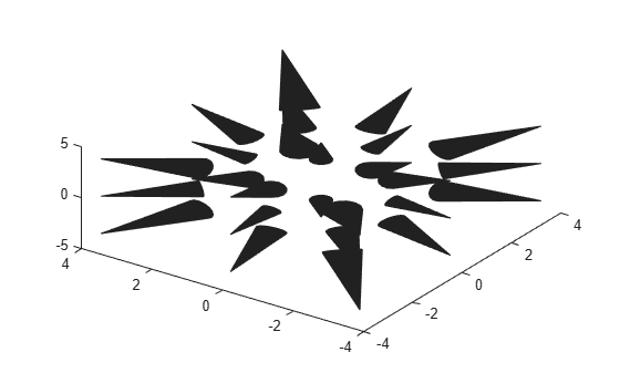
Create a set of vector coordinates and vector components.
[X,Y,Z] = meshgrid(-5:2:5);
U = sign(X);
V = sign(Y);
W = sign(Z);
Create a set of cone coordinates. Then create a cone plot, and return the Patch object p so you can change its properties later. Configure the axes to display a 3-D view.
[Cx,Cy,Cz] = meshgrid(-2:2:2);
p = coneplot(X,Y,Z,U,V,W,Cx,Cy,Cz);
view([305 55])
Change the cone colors by setting the FaceColor property of the Patch object. Remove the patch edges by setting the EdgeColor property of the Patch object to "none". Then give the cones a 3-D appearance by adding a light and displaying the axes grid.
p.FaceColor = "cyan";
p.EdgeColor = "none";
camlight
grid on
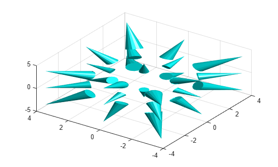
To ensure that the cones have the right proportions, configure the axes to have the same scale in each dimension.
axis equal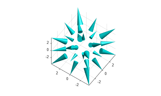
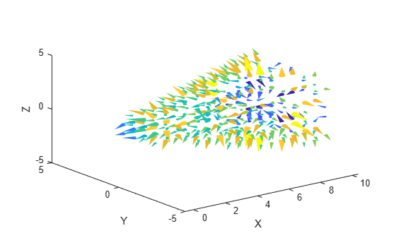
You can use color as an additional dimension for visualizing your data. In this example, create an array that varies the cone colors according to their cross-sectional differences along the lengths of the cones.
Read the flow data set and calculate a set of vector components.
[X,Y,Z,M] = flow(8);
[U,V,W] = gradient(M);
Find the vectors with magnitudes greater than 1. Use the locations of those vectors as the query points for positioning the cones.
mag = sqrt(U.^2 + V.^2 + W.^2);
idx = mag > 1;
Cx = X(idx);
Cy = Y(idx);
Cz = Z(idx);
Create an array colors that contains the cross-sectional differences between the bases and tips of the cones. Create a cone plot, using the colors array to control the colors of the cones. Then configure the axes to display a 3-D view.
Remove the patch edges by setting the EdgeColor property to "none", and display labels for each of the axes.
colors = hypot(Y+V,Z+W) - hypot(Y,Z);
p = coneplot(X,Y,Z,U,V,W,Cx,Cy,Cz,colors);
view(3)
p.EdgeColor = "none";
xlabel("X")
ylabel("Y")
zlabel("Z")
Input Arguments
Output Arguments
Extended Capabilities
Version History
Introduced before R2006a