Adaptive DPD Design: A Top-Down Workflow
By Kerry Schutz, MathWorks
Digital predistortion (DPD) is a baseband signal processing technique that corrects for impairments in RF power amplifiers (PAs). These impairments cause out-of-band emissions or spectral regrowth and in-band distortion, which correlate with an increased bit error rate (BER). Wideband signals with a high peak-to-average ratio, such as those in LTE/4G transmitters, are particulary susceptible to these unwanted effects.
A top-down modeling and simulation approach lets you quickly identify and fix these issues. This article presents a top-down workflow for modeling and simulating PAs and DPDs using MATLAB, Simulink, Signal Processing Toolbox, Control System Toolbox, and DSP System Toolbox. Starting from PA measurements, we derive a static DPD design based on a memory polynomial, which corrects for both the non-linearities and memory effects in the PA. We construct a system-level model to evaluate the DPD's effectiveness. Because PA characteristics vary over time and operating conditions, we transform the static DPD design into an adaptive one. We evaluate two adaptive DPD designs, one based on the Least Mean Square (LMS) algorithm and a second based on the Recurive Predictor Error Method (RPEM) algorithm.
The models used in this article are available for download.
Overview of the Workflow
Our goal is to develop a simulation model that accurately represents the PA's impairments, and an adaptive DPD design that mitigates those impairments1. We divide the modeling effort into five stages:
- Model and simulate the PA
- Derive DPD coefficients
- Evaluate the static DPD design
- Turn the static DPD design into an adaptive one
- Evaluate the LMS and RPEM variants
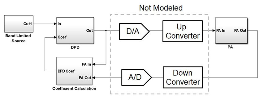
To accelerate the simulations, we will make the following simplifications (Figure 1):
- Model the PA as a discrete time system (in practice, the PA is an analog circuit)
- Model the PA signal as baseband complex (in practice, the PA signal is a real passband signal)
- Use double-precision data types and math (in practice, integer data types and math would be used)
- Omit quantization effects caused by the ADC and DAC
Modeling and Simulating the PA
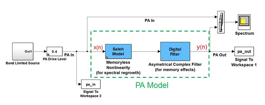
The PA model consists of a Saleh amplifier [3] in series with an asymmetrical complex filter (Figure 2). The excitation is an additive white Gaussian noise (AWGN) signal that has been low-pass elliptic filtered.
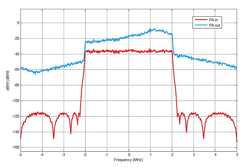
We run the model and log the input and ouput signals, \(x\) and \(y\), respectively, while monitoring their spectrums (Figure 3).
Deriving the DPD Coefficients
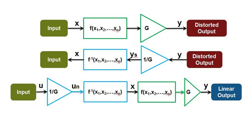
The static DPD design is derived from PA measurements (Figure 4). The top path in Figure 4 represents the PA model. The PA is partitioned into a non-linear function followed by a linear gain G. The middle path shows the PA running in reverse. This path represents the DPD. We cannot run a PA in reverse physically, but we can do so mathematically, and this is the key to the DPD derivation. In reverse, we apply the inverse non-linear operation, \(f^{-1}(x_1,x_2,…x_n)\). The bottom path in Figure 4 is the cascade of the top two paths, namely, the DPD and the PA.
The DPD derivation can now proceed as follows:
-
Assume a memory polynomial [1] form for the PA’s non-linear operator, \(f(x_1,x_2,…x_n)\).
\[y_{MP} (n) = \sum_{k=0}^{K-1}\ \sum_{m=0}^{M-1}\ a_{km} x(n-m) | x(n-m)|^k\]
Equation 1
where
\(x\) is the PA input
\(y\) is the PA output
\(a^{km}\) are the PA polynomial coefficients
\(M\) is the PA memory depth
\(K\) is the degree of PA non-linearity
\(n\) is the time indexThe input \(x\), the output \(y\), and the coefficients \(a^{km}\) are complex valued.
-
Reverse the roles of \(x\) and \(y\) in \(1\) to model the DPD’s inverse non-linear function, \(f_{-1}(x_1,x_2,…x_n)\).
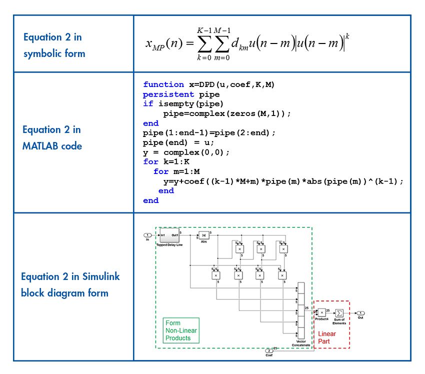
\[x_{MP} (n) = \sum_{k=0}^{K-1}\ \sum_{m=0}^{M-1}\ d_{km}y_{ss}(n-m) |y_{ss}(n-m)|^k\]
Equation 2
Note that \(y(n)\) has been normalized by the linear gain \(G\) and optionally time shifted.
\[y_s(n) = y(n)/G\] \[y_{ss}(n) = y_s(n+\text{offset})\]
where offset is a fixed positive integer.
Timing alignment is critical. If the PA has significant memory requirements, we might need to offset \(y\) in time before deriving the coefficients. The DPD must correctly account for the PA’s positive delay. No realizeable structure can possess negative delay, but you can derive the coefficients based on a time shift in the PA output. And, remember, the PA output is an input in the DPD coefficient derivation. This means that you can make the output \(x\) respond to the input \(y\) “offset” samples earlier by basing the coefficient derivation on a new sequence, \(y_{ss}(n) = y_s(n+\text{offset})\) . In our example, we use an offset of three samples.
-
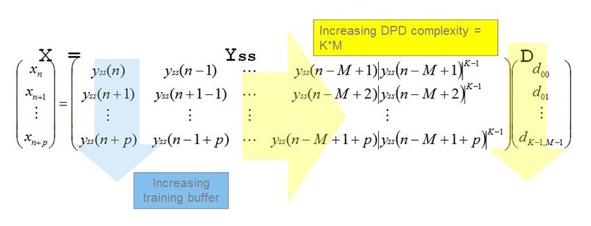
Solve for the DPD coefficients, \(d_{km}\). We rewrite equation 2 as a set of system of linear equations (Figure 5). Solving for \(d_{km}\) then amounts to solving an over-determined system of linear equations, equation 3.
The measurements \(x\) and \(y\) are knowns. A certain value for \(K\) and \(M\) is chosen based on the complexity of the PA. We chose \(M=K=5\) and thus solved for \(K*M = 25\) complex coefficients.
\[d_{km} = Y_{ss} \setminus X \]
Equation 3
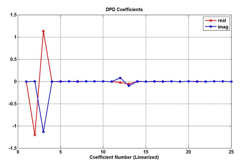
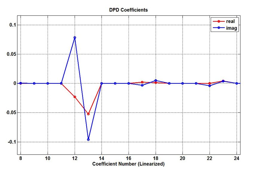
We use the MATLAB backslash operator to solve this over-determined system of equations for the DPD coefficients \(d_{km}\) and the results are shown in Figures 6 and 7.
Evaluating the Fixed-Coefficient DPD Design
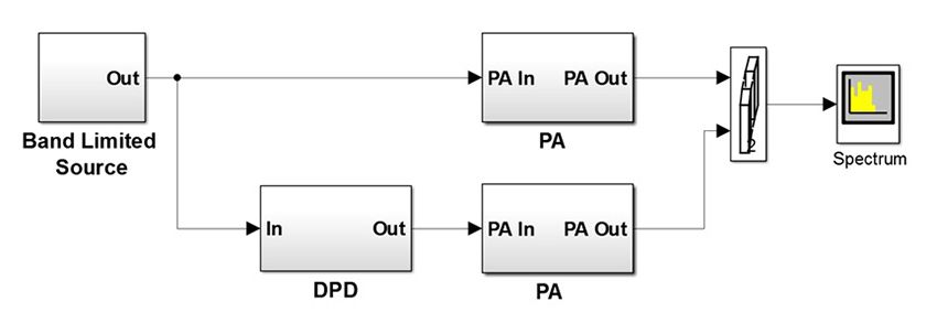
To evaluate the design, we created a system model of the DPD and PA (Figure 8).
The first task is implementing equation 2. It is straightforward to represent these equations in MATLAB, as shown in Table 1.
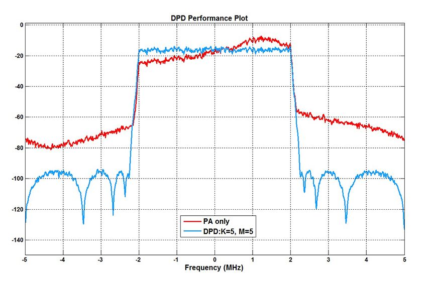
The results of simulating the verification model for \(K=M=5\) is shown in Figure 9.
Going Adaptive
Although our DPD design shows promise, it does not lend itself well to an adaptive implementation. Additionally, the matrix inverse math and the large buffers required to solve an over-determined system of equations are not feasible for hardware implementation.
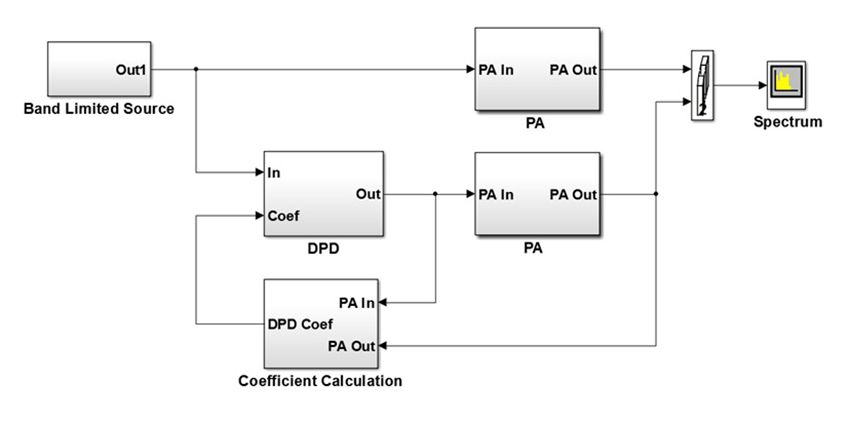
We used an indirect learning architecture [2] to implement an adaptive DPD (Figure 10). The design consists of a Coefficient Calculation subsystem and a DPD subsystem. It is a streaming implementation with no matrix inverse.
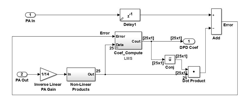
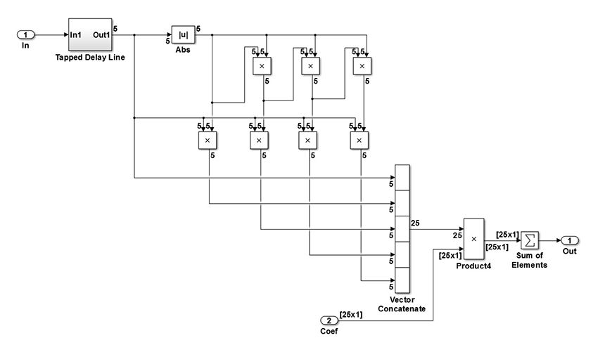
The DPD subsystem is identical in form to that shown in Table 1. Here we focus on the Coefficient Calculation subsystem (Figure 11).
The adaptive DPD architecture has two copies of the DPD algorithm, one for learning the coefficients and the other for implementing them. The combination of the NonLinear_Prod (Figure 12) and Coef_Compute subsystems implement the learning copy of the DPD subsystem.
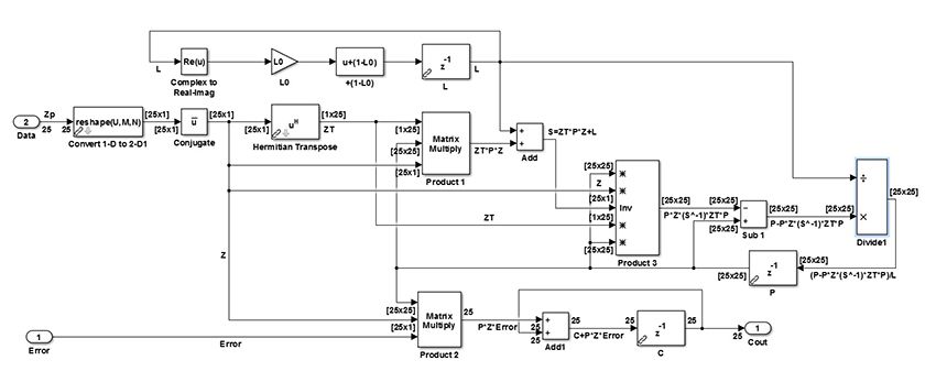
The DPD coefficients, \(d_{km}\), are computed using either the LMS algorithm (Figure 13) or the recursive predictor error method (RPEM) algorithm (Figure 14) . The LMS algorithm is relatively simple in terms of the required resources. The RPEM-based coefficient computation is far more complex than the LMS2.
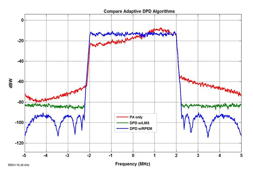
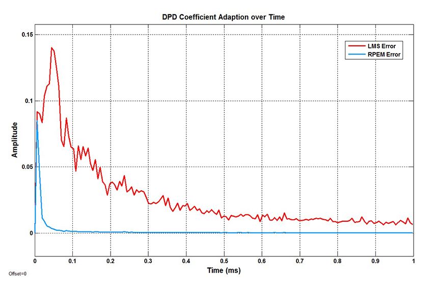
Both the LMS and RPEM algorithms compute an error signal in a feedback loop. The error is the difference between the measured PA input and the estimated PA input. The algorithm attempts to drive this error to zero and in doing so converge on a best estimate of the DPD coefficients. We compare the performance of the two methods (Figures 15 and 16).
The RPEM method provides significantly better results in terms of both spectral growth reduction and rate of convergence.
The RPEM algoritm converges to the same set of coefficients as those computed from off-line PA measurements, while the LMS algorithm never quite converges to this ideal solution. The RPEM algorithm does have disadvantages, however. The RPEM algorithm using \(M = K = 5\) requires approximately 75,300 multiplies per update. The LMS algorithm for the same \(M\) and \(K\) requires approximately 100 multiplies per update. The RPEM algorithm is thus 753 times more computationally expensive. In its current form the RPEM algorithm is not well suited for hardware implementation. On the other hand, the LMS-based approach is much better suited to hardware implementation but is relatively lacking in spectral regrowth reduction.
Summary
This article demonstrates a workflow for modeling and simulating PAs and DPD. We show the DPD design process progressing from an offline batch processing derivation involving matrix inverse computations to a fully streaming and adaptive implementation involving no matrix inverses. We use three figures of merit to evaluate the adaptive DPD design’s effectiveness: spectral regrowth reduction, rate of convergence, and computational complexity. We compare two variants of the adaptive indirect learning architecture, one based on the LMS algorithm and the second based on the RPEM algorithm. The RPEM algorithm is shown to be superior in terms of spectral regrowth reduction and rate of convergence but prohibitive in terms of computational cost.
We use a combination of MATLAB and Simulink for this project. MATLAB is used to define system parameters, test individual algorithms, and perform offline compuations. Simulink is used to integrate the individual PA and DPD components into a test harness where feedback loops, data sizes, and design partitions are easily discerned.
1 The models shown in this article are based on [1] and [2].
2The RPEM algorithm is summarized in equation 24 in [2].
Published 2014 - 92128v00
References
-
Morgan, Ma, Kim, Zierdt, and Pastalan. “A Generalized Memory Polynomial Model for Digital Predistortion of RF Power Amplifiers.” IEEE Trans. on Signal Processing, Vol. 54, No. 10, Oct. 2006.
-
Li Gan and Emad Abd-Elrady. “Digital Predistortion of Memory Polynomial Systems Using Direct and Indirect Learning Architectures.”Institute of Signal Processing and Speech Communication, Graz University of Technology.
-
Saleh, A.A.M., "Frequency-independent and frequency-dependent nonlinear models of TWT amplifiers." IEEE Trans. Communications, vol. COM-29, pp.1715-1720, November 1981.
