Computing π
By Cleve Moler, MathWorks
Computing hundreds, or trillions, of digits of π has long been used to stress hardware, validate software, and establish bragging rights. MATLAB® implementations of the most widely used algorithms for computing π illustrate two different styles of arithmetic available in Symbolic Math Toolbox™: exact rational arithmetic and variable-precision floating-point arithmetic.
Last August, two computer hobbyists, Alexander Yee and Shigeru Kondo, announced that they had set a world record by computing 5 trillion digits of π (Figure 1). Their computation took 90 days on a “homebrew” PC. Yee is now a graduate student at the University of Illinois. His computing software, “y-cruncher,” began as a class project at Palo Alto High School. Kondo is a systems engineer who assembles personal computers at his home in Japan. The machine that he built for this project (Figure 2) has two Intel® Xeon® processors with a total of 12 cores, 96 gigabytes of RAM, and 20 external hard disks with a combined capacity of 32 terabytes.

Figure 1. A log plot of the data from the Wikipedia article “Chronology of computation of pi” showing how the world record for number of digits has increased over the last 60 years. A linear fit to the logarithm reveals a Moore’s Law phenomenon. The number of digits doubles about every 22.5 months.
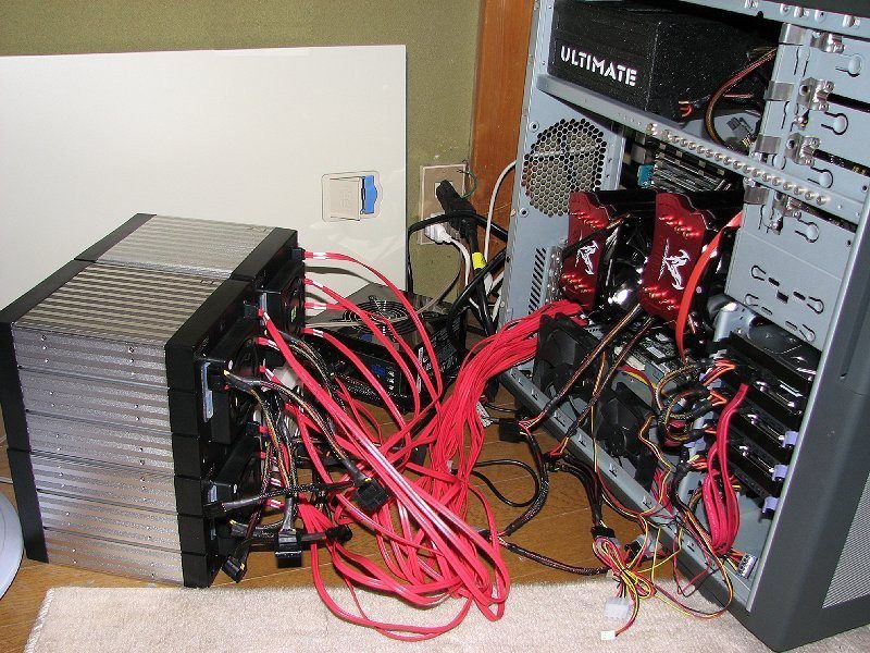
Figure 2. Shigeru Kondo’s homebrew PC, which currently holds the world record for computing digits of π.
The computation of 5 trillion digits is a huge processing task where the time required for the data movement is just as important as the time required for the arithmetic.
y-cruncher uses several different formulas for computation and verification. The primary tool is a formidable formula discovered by David and Gregory Chudnovsky in 1987:
\[\frac{1}{\pi} = 12 \sum_{k=0}^{\infty} \left(-1\right)^{k}\frac{(6k)!(13591409 + 545140134k)}{(3k)!(k!)^{3}(640320)^{3k+\frac{3}{2}}}\]
The Chudnovsky brothers, who were the subject of two fascinating articles in The New Yorker and a NOVA documentary, have also built homebrew computers in their apartment in Manhattan. The massively parallel machine that they assembled from commodity parts in the 1990s was considered a supercomputer at the time.
High-Precision Arithmetic in Symbolic Math Toolbox
Symbolic Math Toolbox provides two styles of high-precision arithmetic: sym and vpa.
The sym function initiates exact rational arithmetic: Arithmetic quantities are represented by quotients and roots of large integers. Integer length increases as necessary, limited only by computer time and storage requirements. Quotients and roots are not computed unless the result is an exact integer.
The vpa function initiates variable-precision floating-point arithmetic: Arithmetic quantities are represented by decimal fractions of a specified length together with a power-of-10 exponent.
Arithmetic operations, including divisions and roots, can involve roundoff errors at the level of the specified accuracy. For example, the MATLAB statement
p = rat(pi)
produces three terms in the continued fraction approximation of π
p = 3 + 1/(7 + 1/16)
Then the statement
sym(p)
yields the rational expression
355/113
which is an attractive alternative to the familiar 22/7. On the other hand, the statement
vpa(p,8)
produces the 8-digit floating-point value
3.1415929
The Chudnovsky Algorithm
Our MATLAB programs implement three of the hundreds of possible algorithms for computing π. The Chudnovsky algorithm (Figure 3) uses exact rational arithmetic until the last step.
 function P = chud_pi(d)
 % CHUD_PI Chudnovsky algorithm for pi.
 % chud_pi(d) produces d decimal digits.

 k = sym(0);
 s = sym(0);
 sig = sym(1);
 n = ceil(d/14);
 for j = 1:n
     s = s + sig * prod(3*k+1:6*k)/prod(1:k)^3 * ...
     (13591409+545140134*k) / 640320^(3*k+3/2);
     k = k+1;
     sig = -sig;
 end
 S = 1/(12*s);
 P = vpa(S,d);
Figure 3. MATLAB implementation of the Chudnovsky algorithm, using sym to initiate exact rational arithmetic.
Each term in the Chudnovsky series provides about 14 decimal digits, so to obtain digits requires [ ] terms. For example, the statement
chud_pi(42)
uses exact rational computation to produce
\[\frac{3405449678154416971853498155008000000\sqrt{640320}}{867407410133324147761288805130794983129}\]
and then the final step uses variable-precision floating-point arithmetic with 42 digits to produce
3.14159265358979323846264338327950288419717
One interesting fact about the digits of π is revealed by
chud_pi(775)
or
vpa(pi,775)
These both produce 775 digits, beginning and ending with
3.141592653589793238 ...... 707211349999998372978
We see not only that chud_pi is working correctly but also that there are six 9s in a row around position 765 in the decimal expansion of π (Figure 4).

Figure 4. 10,000 digits of π, visualized in MATLAB. Can you see the six consecutive 9s in the eighth row?
Computing 5000 digits with chud_pi requires 358 terms and takes about 20 seconds on my laptop. The final symbolic expression contains 12,425 characters.
The Algebraic-Geometric Mean Algorithm
The Chudnovsky formula is a power series: Each new term in the partial sum adds a fixed number of digits of accuracy. The algebraic-geometric mean algorithm is completely different; it is quadratically convergent: Each new iteration doubles the number of correct digits. The agm algorithm has a long history dating back to Gauss and Legendre. Its ability to compute π was discovered independently by Richard Brent and Eugene Salamin in 1975.
The arithmetic mean of two numbers, \((a+b)/2\), is always greater than their geometric mean, \(\sqrt{ab}\) . Their arithmetic-geometric mean, or \(agm(a,b)\), is computed by repeatedly taking arithmetic and geometric means. Starting with \(a_0 = a\) and \(b_0 = b\), iterate
\[\begin{align} a_{n+1} & = \frac{a_n + b_n}{2} \\ b_{n+1} & = \sqrt{a_{n}b_{n}}\end{align}\]
until \(a_n\) and \(b_n\) agree to a desired accuracy. For example, the arithmetic mean of 1 and 9 is 5, the geometric mean is 3, and the agm is 3.9362.
The powerful properties of the agm lie not just in the final value but also in the results generated along the way. Computing \(\pi\) is just one example. It involves computing
\[M = agm\left(1,\frac{1}{\sqrt{2}}\right)\]
During the iteration, keep track of the changes,
\[c_n = a_{n+1} - a_n\]
Finally, let
\[S = \frac{1}{4}\sum_{n=0}^{\infty} 2^n c_{n}^{2}\]
Then
\[\pi = \frac{M^2}{S}\]
Our MATLAB function for the agm algorithm (Figure 5) uses variable-precision floating-point arithmetic from the very beginning. If we used symbolic rational arithmetic, we would end up with a nested sequence of square roots. After just two iterations we would have
\[\frac{\left(\frac{\sqrt{\frac{\sqrt{2}}{2}}}{2} + \frac{\sqrt{2}}{8} + \frac{1}{4}\right)^2}{\frac{1}{4} - \left(\frac{\sqrt{2}}{4} - \frac{1}{2}\right)^2 - 2\left(\frac{\sqrt{2}}{8} - \frac{\sqrt{\frac{\sqrt{2}}{2}}}{2} + \frac{1}{4}\right)^2}\]
The decimal value of this monstrosity is 3.14168, so it is not yet a very good approximation to π. The complexity doubles with each iteration.
 function P = agm _ pi(d)
 % AGM _ PI Arithmetic-geometric mean for pi.
 % agm _ pi(d) produces d decimal digits.
 digits(d)
 a = vpa(1,d);
 b = 1/sqrt(vpa(2,d));
 s = 1/vpa(4,d);
 p = 1;
 n = ceil(log2(d));
 for k = 1:n
     c = (a+b)/2;
     b = sqrt(a*b);
     s = s - p*(c-a)^2;
     p = 2*p; a = c;
 end
 P = a^2/s;
Figure 5. MATLAB implementation of the arithmetic-geometric mean algorithm, using digits and vpa to initiate variable-precision floating-point arithmetic.
Such exact symbolic expressions are computationally unwieldy and inefficient. With vpa, however, the quadratic convergence can be seen in the successive iterates:
 3.2
 3.142
 3.1415927
 3.141592653589793
 3.1415926535897932384626433832795
 3.1415926535897932…79502884197169399375105820974944592
The sixth entry in this output has 64 correct digits, and the tenth has 1024.
The quadratic convergence makes agm very fast. To compute 100,000 digits requires only 17 steps and about 2.5 seconds on my laptop.
The BBP Formula
Yee spot-checked his computation with the BBP formula. This formula, named after David Bailey, Jonathan Borwein, and Simon Plouffe and discovered by Plouffe in 1995, is a power series involving inverse powers of 16:
\[\pi = \sum_{k=0}^{\infty} \left(\frac{4}{8k + 1} - \frac{2}{8k + 4} - \frac{1}{8k + 5} - \frac{1}{8k + 6}\right)\left(\frac{1}{16}\right)^k\]
The remarkable property of the BBP formula is that it allows the computation of several consecutive hexadecimal digits in the base 16 expansion of \(\pi\) without computing the earlier digits and without using extra-precision arithmetic. A formula for the hex digits starting at position \(d\) is obtained by simply multiplying this formula by \(16^d\) and then taking the fractional part.
I can’t resist concluding that BBP can be used to compute just a piece of \(\pi\).
Our BBP program is too long to be included here, but all three programs, chudovsky_pi, agm_pi, and bbp_pi, are available for download on MATLAB Central.
Published 2011 - 91954v00
References
-
Alexander J. Yee and Shigeru Kondo, “5 Trillion Digits of Pi,” August 2, 2010.
-
Richard Preston, “The Mountains of Pi,” The New Yorker, March 2, 1992.
-
Richard Preston, “Capturing the Unicorn,” The New Yorker, April 11, 2005.
-
“Brothers Chudnovsky,” PBS, NOVA, July 26, 2005.
-
David Bailey, Jonathan Borwein, Peter Borwein, and Simon Plouffe, “The Quest for Pi,” Mathematical Intelligencer 19, pp. 50-57, 1997.
-
Jonathan M. Borwein and David H. Bailey, Mathematics by Experiment: Plausible Reasoning in the 21st Century, AK Peters, Natick, MA, 2008.
-
“Chronology of computation of pi,” Wikipedia, March 9, 2011.