Making All the Right Noises: Shaping Sound with Audio Beamforming

At Philips Research, we have developed technology that enables two people in the same room to hear the same audio output at different volumes. Based on audio beamforming, this technology is a new application of an old idea, made possible by the falling cost of computing power. We were granted a patent for our audio beamforming technology in 2012.

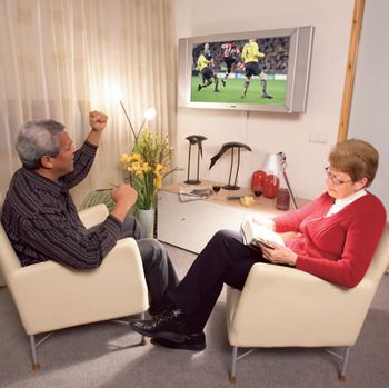
Imagine two people in a room watching television—say, the Netherlands winning in the World Cup (Figure 1). One is slightly deaf and needs the volume high, but the other isn’t interested in soccer and wants the volume low. This effect could be achieved by mounting several speakers throughout the room, but this solution would require unsightly trailing wires and time-consuming installation. Getting the same result from a single array of speakers mounted on the TV is an attractive alternative, but is technically challenging. We addressed that challenge by creating a detailed MATLAB^® simulation that provided us with a means of calculating the loudspeaker parameters we needed for beamforming.

The Audio Beamforming System

Our audio beamforming system consists of a loudspeaker array with each speaker in the array controlled by a digital signal processor (DSP). The DSP uses a FIR filter and other signal processing algorithms to control the loudspeaker output. Our challenge was to identify the FIR filter coefficients that would produce the desired volume at different points in the room.

To describe this system mathematically, we defined a matrix G(ω) that described the sound propagation of each individual speaker in the system in each individual direction (an MxN matrix) at different frequencies ω. If the set of loudspeaker coefficients is H(ω), we express the total response of the system as

\[\begin{equation}L(\omega) = G(\omega)H(\omega)\end{equation}\tag{1}\]

Each user in the room will control their volume using a remote control that identifies their position, so we can calculate the target response we want \(T\). We want \(L\) to be close to \(T\), so we’re minimizing \(L(\omega) - T\), or

\[\begin{equation}\min_{H(\omega)}(\|G(\omega)H(\omega) - T\|)\end{equation}\tag{2}\]

To solve this matrix equation, we turned to MATLAB.

It would be possible to solve this matrix equation in C, but it would be very time-consuming. We would have to write and test matrix calculation code, and write our own visualization functions, such as polar plots. With MATLAB and Signal Processing Toolbox™, we have access to advanced and thoroughly tested matrix algebra functions, as well as extensive graph plotting and visualization capabilities.

Since audio research work involves a great deal of trial and error, for us another advantage of working in MATLAB is the ability to try out different design ideas. As a compiled language, C does not lend itself to this way of working. Each time we want to try out a new function, we have to recompile code and recreate the data. By contrast, MATLAB can work interactively, enabling us to apply different functions and immediately visualize their effect on the system. This step-by-step interactivity makes MATLAB a great deal easier and faster to use than C.

Developing the Audio Processing Toolbox

During my research work at Delft University of Technology, I developed tools for modeling audio processing applications in MATLAB, including simulating sound propagation in rooms. I wanted to apply these tools to the audio beamforming project, but my colleagues and I soon realized that it was too complex a problem for my tools to handle. We therefore spent time developing the tools into a Philips Research audio processing toolbox for MATLAB. Our MATLAB audio toolbox, which includes a range of specialist custom functions, simulates sound fields for arbitrary loudspeaker systems and models arbitrary processing within the system. It enabled us to model the effect of different FIR filters and delays at each speaker in an array using a complex transfer function.

Optimizing the System for Stability and Efficiency

The success of the beamforming project relied on producing an acoustical field \(L\) as close as possible to a target field \(T\), which means solving equation 2. Using the optimization features of MATLAB made this task straightforward, but in solving the equation we also had to take account of other factors, in particular, system stability and efficiency.

In an unstable system, small changes in the system parameters can lead to large changes in the system output. Unfortunately, there will be many small changes between our initial modeled system and the real system. The production process introduces variations in, for example, speaker sensitivity and response, and small changes such as a slightly different choice of loudspeaker or speaker layout could be introduced later in the design process. We want to produce a solution that is robust, one in which small variations change the output by a small amount.

An inefficient system relies on high speaker volumes. The net result is high power consumption with low audio output, which means using higher-powered—and more expensive—speakers and amplifiers. We constrain our optimization to produce solutions that do not exhibit this behavior.

Our MATLAB tools used optimization with these constraints to produce a stable and efficient solution for \(H(\omega)\), from which we calculated FIR coefficients and other parameters for each loudspeaker. In practice, we selected individual loudspeaker filter coefficients that together provided a good match with the target while ensuring stability and efficiency.

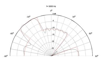
Even though our optimization was highly constrained, we were able to get very close to our target (Figure 2), and the solution was both stable and efficient.

Enhancing the Model

We began our research with a proof-of-concept model consisting of a simple loudspeaker frequency response in our transfer function. As the project matured, we included more sophisticated and realistic speaker frequency responses. In cases where we knew which speaker we were going to be using, we included the measured loudspeaker frequency responses. If this data wasn’t available (perhaps because the speaker hadn’t yet been built), we used a theoretical response, derived from a MATLAB model.

Testing the System Behavior

Using the MATLAB audio toolbox, we tested the performance of our loudspeaker parameters using sound propagation simulation. We entered the room characteristics (length, width, height, and loudspeaker locations) into our models and converted the frequency-domain output data to a time-domain model. We configured the output of the time-domain model as a series of movie frames, which we combined to show an animation of the propagation of the sound wave through the room using the MATLAB movie function.

The animation clearly revealed individual beams and their frequency dependence. At low frequencies, we had little beam formation, which is acceptable because the type of content we would like to beam (e.g., TV commentary) typically has relatively little energy at very low frequencies anyway. At higher frequencies we saw additional unwanted beams forming. We examined the results to find out whether these extra beams would cause effects audible to users.

Because the output of our modeling work includes a complex transfer function for every point in the room, we ran one further check on the behavior of the system. We took the response at two points spaced about 20 cm apart (the width of a human head) and convolved the response with a real audio signal, such as music or a television commentary. We then output the results of our MATLAB calculations as an audio stream and listened to the result. These simulations enabled us to hear what the real audio would sound like at any point in the room, giving us insight into the system’s sound quality and intensity.

As well as varying the sound level at different points in the room, we can use this same technology to feed different audio signals to different parts of the room. One person can listen to classical music while another listens to a TV program. We can place the different sound channels anywhere in the room.

Ongoing Audio Research

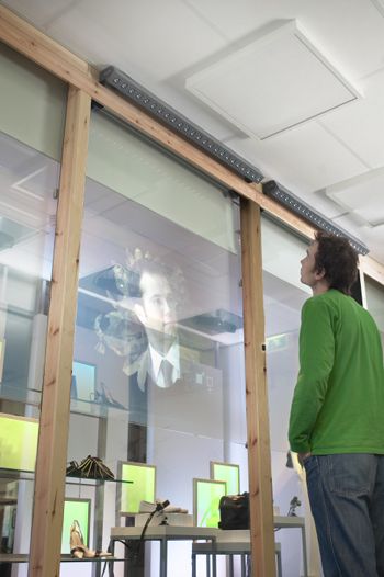
The combination of MATLAB simulation and low-cost digital signal processing is making it possible to create brand new products using audio beamforming. A recent project applies audio beamforming to an audio-visual device on display in a shopping mall (Figure 3). With audio beamforming technology, we can direct the sound to the person who is interacting with the display, or even have a separate audio stream for each individual interacting with the system (for example, one stream in English and one in Dutch). Individuals passing by the system, perhaps only two meters or so away, won’t hear a thing.