NR Interference Modeling with Toroidal Wrap-Around
This example shows how to model up to 19-site cluster with toroidal wrap-around, as described in ITU-R M.2101-0. This example uses the system-level channel model specified in 3GPP TR 38.901. The wrap-around provides uniform interference at the cluster edge. All the cells in the cluster operate in the same frequency band with the serving 5G base station node (gNB) at the center of the cell. You can enable or disable the wrap-around to observe that with wrap-around, the performance metrics of an edge cell become similar to the center cell.
Optional Product: This example also demonstrates how to utilize GPU acceleration for the 38.901 channel filtering, in full-PHY modeling, using the Parallel Computing Toolbox™.
Introduction
This example models:
Up to 19-site cluster with three cells/site, giving a total of 57 cells. A site is represented by 3 colocated gNBs with directional antennas covering 120 degrees area (that is, 3 sectors per site).
Co-channel intercell interference with wrap-around modeling for removing edge effects.
System-level channel model based on 3GPP TR 38.901.
Outer loop link adaptation (OLLA) and downlink multi-user MIMO (MU-MIMO).
Downlink shared channel (DL-SCH) data transmission and reception.
DL channel quality measurement using either channel state information reference signal (CSI-RS) or sounding reference signal (SRS).
Uplink shared channel (UL-SCH) data transmission and reception.
UL channel quality measurement by gNBs, based on the SRS received from the UE nodes.
This example assumes that nodes send the control packets (buffer status report (BSR), DL assignment, UL grants, PDSCH feedback, and CSI report) out of band, eliminating the requirement for transmission resources and ensuring error-free reception.
Toroidal Wrap-around Modeling
To simulate the behavior of a cellular network without introducing edge effects, this example models an infinite cellular network by using toroidal wrap-around. The entire network region relevant for simulations is a cluster of 19 sites (shown bold in this figure). The left-hand figure shows the network region of 19 sites without wrap-around. Site 0 of the central cluster, shown in red, is uniformly surrounded and experiences interference from all sides. A cell in an edge site like site 15 experiences less interference. In the right-hand figure, the wrap-around repeats the original cluster six times to uniformly surround the central cluster.
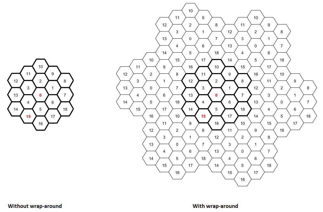
The wrap-around model treats the signal or interference from any UE node to a cell as if that the UE node is in the original cell cluster and the gNB in any of the seven clusters specified in ITU-R M.2101-0. The distances used to compute the path loss from a transmitter node at to a receiver node at is the minimum of these seven distances.
Distance between and
Distance between and , where is the distance between two adjacent gNBs (inter-site distance)
Distance between and
Distance between and
Distance between and
Distance between and
Distance between and
These equations are derived from the equations in ITU-R M.2101-0 Attachment 2 to Annex 1. In 3GPP TR 38.901 and in the figure above, the rings of 6 and 12 sites around the central site are orientated differently from the orientations in ITU-R M.2101-0, so modified equations are required.
If you disable wrap-around, then the distance between nodes is the Euclidean distance.
Scenario Configuration
Create a wireless network simulator.
rng("default"); % Reset the random number generator numFrameSimulation =15; % Simulation time in terms of number of 10 ms frames networkSimulator = wirelessNetworkSimulator.init();
Create cell sites, sectors, and UE nodes in each cell for the urban macro (UMa) scenario.
cellSites =7; % Number of cell sites
isd = 500;                           % Inter-site distance in meters
sectors = 1;      % Number of sectors for each cell site
ues = 4;                             % Number of UEs to drop per cell
% Enabling wrapping is possible for 3 cell sites with 3 sectors each or extend
% to 7 or 19 sites with 1 or 3 sectors per site.
isWrapping = true;   % Enable toroidal wrap-around modeling of cells. Set it to false to disable toroidal wrap-around
phyModeling = "abstract-phy";  % Set to 'full-phy' for full PHY modeling, or 'abstract-phy' for abstract PHY modeling

% Create the scenario builder
scenario = h38901Scenario(Scenario="UMa", FullBufferTraffic="on", NumCellSites=cellSites, ...
    InterSiteDistance=isd, NumSectors=sectors, NumUEs=ues, Wrapping=isWrapping);

% Add cell sites to the network simulator and configure parameters for gNB
gNBs = [];
for i = 1:cellSites
    gNB = addCellSite(scenario, networkSimulator, PHYModel=phyModeling, DuplexMode="TDD", ...
        NumTransmitAntennas=16, NumReceiveAntennas=16, TransmitPower=49, ...
        ChannelBandwidth=5e6, NumResourceBlocks=25, CarrierFrequency=6e9, SRSPeriodicityUE=160);
    gNBs = [gNBs gNB];
end
Configure the link adaptation (LA) parameters. The parameters specify a 10 percent target BLER for the UL and DL configurations.
laConfigDL = struct(StepUp=0.9, StepDown=0.1, InitialOffset=1, ResetOffsetOnCSIReport=false);
laConfigUL = struct(StepUp=0.9, StepDown=0.1, InitialOffset=1, ResetOffsetOnCSIReport=false);
Set the downlink CSI measurement signal type, csiMeasurementSignalDLType, to "SRS".
% Alternatively, you can set it to "CSI-RS". Note that the user-pairing algorithm depends on the selected type of downlink measurement signal csiMeasurementSignalDLType ="SRS";
Configure the DL MU-MIMO structure muMIMOConfiguration by setting these fields. For more information about these fields, see the MUMIMOConfigDL name-value argument of configureScheduler function.
Maximum number of UE nodes paired — 2
Maximum number of layers — 8
Minimum number of RBs — 2
Minimum DL SINR — 20 dB
muMIMOConfiguration = struct(MaxNumUsersPaired=2, MaxNumLayers=8, MinNumRBs=2, MinSINR=20);
Configure the scheduler by specifying the gNBs, DL CSI measurement signal type, LA and MU-MIMO configuration.
configureScheduler(gNBs, CSIMeasurementSignalDL=csiMeasurementSignalDLType, LinkAdaptationConfigDL=laConfigDL, ...
    LinkAdaptationConfigUL=laConfigUL, MUMIMOConfigDL=muMIMOConfiguration)

% Drop UEs into the scenario and configure parameters for UEs
dropUEs(scenario, networkSimulator, PHYModel=phyModeling,...
    NumTransmitAntennas=4, NumReceiveAntennas=4, NoiseFigure=6);
GPU Acceleration
When your system-level simulation requires intensive processing, using a GPU can accelerate the overall simulation time by performing the data-intensive part of the computation on the GPU. Use the gpuFlag to perform computations on the GPU. When set to "off", the simulation runs on the CPU. When set to "on", the simulation uses a GPU (requires Parallel Computing Toolbox™). When set to "auto", the simulation automatically uses a GPU device if a compatible GPU device is available.
GPU acceleration is supported for full-PHY modeling. If needed, you can manually enable or disable GPU usage by setting the gpuFlag option.
gpuFlag = "off"; % GPU is "off" by default if phyModeling=="full-phy" gpuFlag ="auto"; % Use GPU if available end
Setup Channel
Create the system-level channel model for the scenario, and connect it to the simulator. Connect the gNB and UE nodes to the channel.
% Create the channel model
channel = h38901Channel(Scenario="UMa", UseGPU=gpuFlag);

% Connect the channel model to the simulator
addChannelModel(networkSimulator, @channel.channelFunction);

% Connect the gNB and UE nodes to the channel
connectNodes(channel, networkSimulator, scenario);
Logging and Visualization Configuration
Set the enableTraces to true to log the traces. If the enableTraces is set to false, then the simulation does not log traces. However, setting enableTraces to false can speed up the simulation.
enableTraces =  true;
true;Set up scheduling logger and phy logger for the cells of interest.
% Select the cells (that is, the sites and sectors) that require collection of
% traces and metrics.
siteOfInterest = [0 6];
sectorOfInterest = [0 0];

numCellsOfInterest = length(siteOfInterest);

if enableTraces
    simSchedulingLogger = cell(numCellsOfInterest,1);
    simPhyLogger = cell(numCellsOfInterest,1);

    for cellIdx = 1:numCellsOfInterest

        % Obtain the gNB and UE nodes for the cell of interest from the scenario
        % object
        [gNB, UEs] = getNodesForCell(scenario, siteOfInterest, sectorOfInterest, ...
            cellIdx);

        % Create an object to log scheduler traces
        simSchedulingLogger{cellIdx} = helperNRSchedulingLogger(numFrameSimulation, ...
            gNB, UEs);

        % Create an object to log PHY traces
        simPhyLogger{cellIdx} = helperNRPhyLogger(numFrameSimulation, gNB, UEs);

    end
end
Set the number of updates for the metrics plot per second, numMetricPlotUpdates. The example updates the metrics plots.
% This parameter has an impact on simulation time.
numMetricPlotUpdates =100;
Set up metric visualizers.
metricsVisualizer = cell(numCellsOfInterest,1);

for cellIdx = 1:numCellsOfInterest

    % Obtain the gNB and UEs for the cell of interest from the scenario object
    [gNB, UEs] = getNodesForCell(scenario, siteOfInterest, sectorOfInterest, cellIdx);

    % Create visualization object for the MAC and PHY metrics
    metricsVisualizer{cellIdx} = helperNRMetricsVisualizer(gNB, UEs, ...
        RefreshRate=numMetricPlotUpdates, PlotSchedulerMetrics=true, ...
        PlotPhyMetrics=true, CellOfInterest=siteOfInterest(cellIdx));

end
Write the logs to MAT-files. You can use these logs for post-simulation analysis.
simulationLogFile = "simulationLogs";Simulation
Run the simulation for the specified numFrameSimulation frames.
% Calculate the simulation duration (in seconds)
simulationTime = numFrameSimulation * 1e-2;

% Run the simulation
run(networkSimulator, simulationTime);

Simulation Visualization
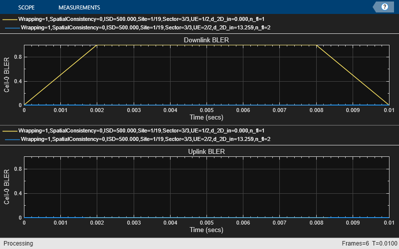
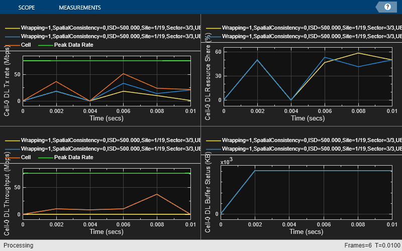
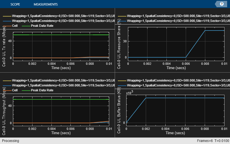
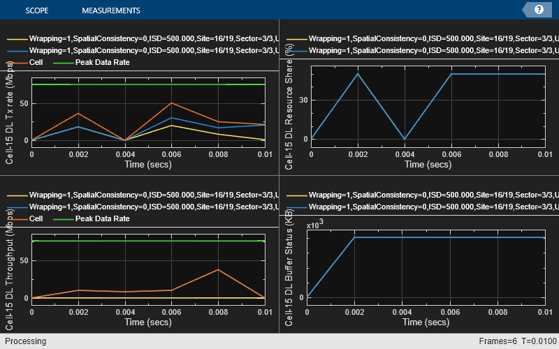
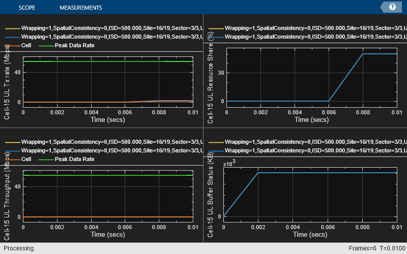
For the cells of interest, run time visualizations show various performance indicators at multiple time steps during the simulation. For a detailed description, see the NR Cell Performance Evaluation with MIMO example.
At the end of the simulation, compare the achieved values for system performance indicators with theoretical peak values (considering zero overheads). Performance indicators displayed are achieved data rate (UL and DL), achieved spectral efficiency (UL and DL), and block error rate (BLER) observed for UEs (UL and DL). The calculated peak values are in accordance with 3GPP TR 37.910.
Note that to get meaningful results, the simulation has to be run for a longer duration and for a larger number of UE nodes per cell.
for cellIdx = 1:numCellsOfInterest

    fprintf("\n\nMetrics for site %d, sector %d :\n\n",siteOfInterest(cellIdx), ...
        sectorOfInterest(cellIdx));

    displayPerformanceIndicators(metricsVisualizer{cellIdx});

end
Metrics for site 0, sector 0 :
Peak UL throughput: 51.55 Mbps
Achieved cell UL throughput: 7.20 Mbps
Achieved UL throughput for each UE: [0.87        1.37        0.04        4.92]
Peak UL spectral efficiency: 10.31 bits/s/Hz
Achieved UL spectral efficiency for cell: 1.44 bits/s/Hz
Block error rate for each UE in the UL direction: [0.017        0.19       0.586       0.138]

Peak DL throughput: 71.10 Mbps
Achieved cell DL throughput: 17.65 Mbps
Achieved DL throughput for each UE: [1.46        6.14        0.39        9.66]
Peak DL spectral efficiency: 14.22 bits/s/Hz
Achieved DL spectral efficiency for cell: 3.53 bits/s/Hz
Block error rate for each UE in the DL direction: [0.034           0       0.022           0]
Metrics for site 6, sector 0 :
Peak UL throughput: 51.55 Mbps
Achieved cell UL throughput: 4.85 Mbps
Achieved UL throughput for each UE: [3.72        0.74        0.14        0.25]
Peak UL spectral efficiency: 10.31 bits/s/Hz
Achieved UL spectral efficiency for cell: 0.97 bits/s/Hz
Block error rate for each UE in the UL direction: [0       0.241       0.052       0.034]

Peak DL throughput: 71.10 Mbps
Achieved cell DL throughput: 5.02 Mbps
Achieved DL throughput for each UE: [0.52        3.19        0.22        1.08]
Peak DL spectral efficiency: 14.22 bits/s/Hz
Achieved DL spectral efficiency for cell: 1.00 bits/s/Hz
Block error rate for each UE in the DL direction: [0.371       0.056        0.09           0]
Simulation Logs
Save the simulation logs related to cells of interest into a MAT file. For a description of the simulation logs format, see the NR Cell Performance Evaluation with MIMO example.
if enableTraces
    simulationLogs = cell(numCellsOfInterest,1);

    for cellIdx = 1:numCellsOfInterest
        % Obtain the gNB for the cell of interest from the scenario object
        gNB = getNodesForCell(scenario,siteOfInterest,sectorOfInterest,cellIdx);

        if gNB.DuplexMode == "FDD"
            logInfo = struct("DLTimeStepLogs",[],"ULTimeStepLogs",[], ...
                "SchedulingAssignmentLogs",[],"PhyReceptionLogs",[]);
            [logInfo.DLTimeStepLogs,logInfo.ULTimeStepLogs] = ...
                getSchedulingLogs(simSchedulingLogger{cellIdx});
        else % TDD
            logInfo = struct("TimeStepLogs",[],"SchedulingAssignmentLogs",[], ...
                "PhyReceptionLogs",[]);
            logInfo.TimeStepLogs = getSchedulingLogs(simSchedulingLogger{cellIdx});
        end

        % Obtain the scheduling assignments log
        logInfo.SchedulingAssignmentLogs = getGrantLogs(simSchedulingLogger{cellIdx});

        % Obtain the phy reception logs
        logInfo.PhyReceptionLogs = getReceptionLogs(simPhyLogger{cellIdx});

        simulationLogs{cellIdx} = logInfo;
    end

    % Save simulation logs in a MAT-file
    save(simulationLogFile, "simulationLogs");
end
Local Functions
function [gNB,UEs] = getNodesForCell(scenario, siteOfInterest, sectorOfInterest, cellIdx)
    siteIdx = siteOfInterest(cellIdx) + 1;
    sectorIdx = sectorOfInterest(cellIdx) + 1;
    numCellSites = numel(scenario.CellSites);

    if (siteIdx > numCellSites)
        warning("The cell site of interest (%d) does not exist, using the last cell site (%d).", ...
            siteIdx-1,numCellSites-1);
        siteIdx = numCellSites;
    end

    numSectors = numel(scenario.CellSites(siteIdx).Sectors);

    if (sectorIdx > numSectors)
        warning("For cell site %d, the sector of interest (%d) does not exist, using the last sector (%d).", ...
            siteIdx-1,sectorIdx-1,numSectors-1);
        sectorIdx = numSectors;
    end

    gNB = scenario.CellSites(siteIdx).Sectors(sectorIdx).BS;
    UEs = scenario.CellSites(siteIdx).Sectors(sectorIdx).UEs;
end
References
[1] 3GPP TS 38.104. “NR; Base Station (BS) radio transmission and reception.” 3rd Generation Partnership Project; Technical Specification Group Radio Access Network.
[2] 3GPP TS 38.214. “NR; Physical layer procedures for data.” 3rd Generation Partnership Project; Technical Specification Group Radio Access Network.
[3] 3GPP TS 38.321. “NR; Medium Access Control (MAC) protocol specification.” 3rd Generation Partnership Project; Technical Specification Group Radio Access Network.
[4] 3GPP TS 38.322. “NR; Radio Link Control (RLC) protocol specification.” 3rd Generation Partnership Project; Technical Specification Group Radio Access Network.
[5] 3GPP TS 38.323. “NR; Packet Data Convergence Protocol (PDCP) specification.” 3rd Generation Partnership Project; Technical Specification Group Radio Access Network.
[6] 3GPP TS 38.331. “NR; Radio Resource Control (RRC) protocol specification.” 3rd Generation Partnership Project; Technical Specification Group Radio Access Network.
[7] 3GPP TR 37.910. “Study on self evaluation towards IMT-2020 submission.” 3rd Generation Partnership Project; Technical Specification Group Radio Access Network.
See Also
Objects
wirelessNetworkSimulator(Wireless Network Toolbox) |nrGNB|nrUE