Optimize Custom Antenna using TR-SADEA Optimizer
This example shows how to optimize a custom antenna using the TR-SADEA optimizer. The example maximizes gain of a custom antipodal Vivaldi antenna at 5 GHz, while limiting the return loss to –10 dB or less. A TR-SADEA optimizer belongs to the class of surrogate-assisted optimizers that use mathematical models to replace time-consuming electromagnetic (EM) simulations. TR-SADEA optimizer enables faster optimization through efficient exploration of search space.
Define Geometry Parameters of Antipodal Vivaldi Antenna
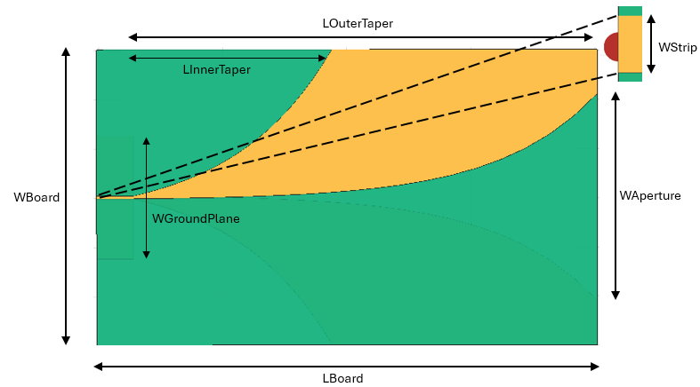
Define dimensions of the aperture, feed line, inner and outer edge taper, ground plane, and circuit board.
baseDimensions = struct;
baseDimensions.ROpening = 30; % Opening rate of taper
baseDimensions.WAperture = 0.024; % Width of the aperture in meter
baseDimensions.WStrip = 0.0021; % Width of the feed line in meter
baseDimensions.LInnerTaper = 0.187; % Length of inner edge taper in meter
baseDimensions.LOuterTaper = 0.08; % Length of outer edge taper in meter
baseDimensions.WGroundPlane = 0.05; % Width of the ground plane in meter
baseDimensions.LBoard = 0.2020; % Length of the printed circuit board in meter
baseDimensions.WBoard = 0.12; % Width of the printed circuit board in meter
baseDimensions.N = 30; % Number of points along taper
Set the taper opening rate to 'ROpening', aperture width to 'WAperture', and feed width to 'Wstrip'. Use these design variables for the optimization. Create the antipodal Vivaldi antenna using the createVivaldi function defined in the Supporting Functions section. View the antenna.
designVariables = [baseDimensions.ROpening,baseDimensions.WAperture,baseDimensions.WStrip];
ca = createVivaldi(designVariables,baseDimensions);
figure
show(ca)
title("Antipodal Vivaldi Antenna")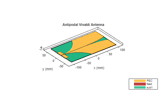
Plot Radiation Pattern
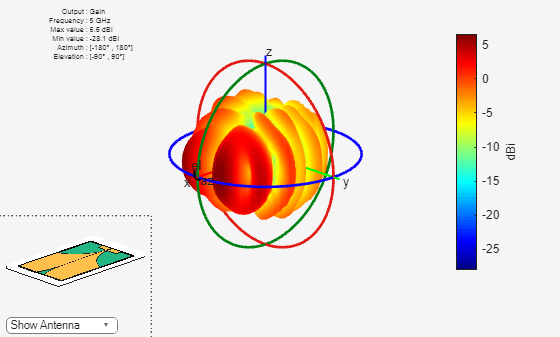
Plot the radiation pattern of this antenna at 5 GHz and observe the gain. The current design yields a maximum gain of around 6 dBi.
pattern(ca,5e9);
Plot Reflection Coefficient
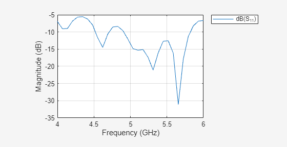
Plot the reflection coefficient of the antenna in the 4 to 6 GHz frequency band with a reference impedance of 50 ohms.
freq = 1e9;
freqRange = linspace(freq*4,freq*6,30);
sparam = sparameters(ca,freqRange);
rfplot(sparam);
Optimize Antenna for Maximum Gain
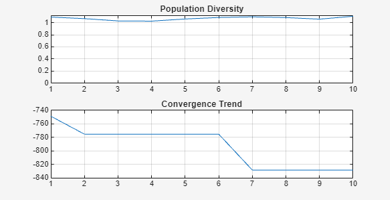
Use the OptimizerTRSADEA object to optimize this antenna. The OptimizerTRSADEA object gives you access to the TR-SADEA optimizer provided in the Antenna Toolbox™. To initialize the OptimizerTRSADEA object, provide the lower and upper bounds of the chosen design variables as input arguments to the OptimizerTRSADEA object creation function. Use the customEvaluation function defined in the Supporting Functions section to set the evaluation criteria for the optimization. Use the optimizeWithPlots function with 10 iterations to optimize the antenna.
s = OptimizerTRSADEA([20 0.03 0.002;30 0.11 0.003]);
s.CustomEvaluationFunction = @customEvaluation;
s.optimizeWithPlots(10);
Use the getBestMemberData function to fetch the optimized values for the design variables.
bestData = s.getBestMemberData;
optimized_values = bestData.member;
Use the optimized values of the design variables to create the optimized antenna.
ca = createVivaldi(optimized_values,baseDimensions);
figure
show(ca)
title("Optimized Antipodal Vivaldi Antenna")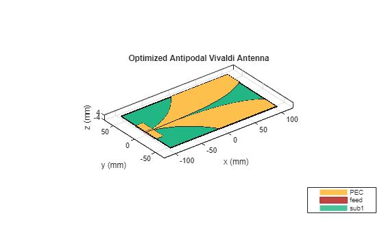
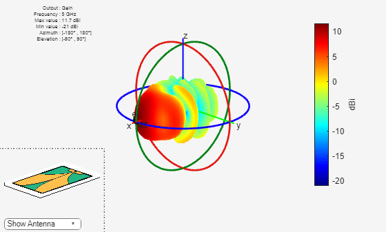
Plot Radiation Pattern of Optimized Antenna
Plot the radiation pattern of the optimized antenna at 5 GHz, and observe the gain. The optimized design yields an improvement in the gain over the original design.
pattern(ca,5e9);
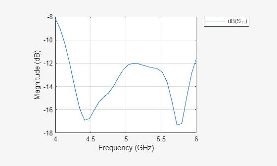
Plot Reflection Coefficient of Optimized Antenna
Plot the reflection coefficient of the optimized antenna in the 4 to 6 GHz frequency band with a reference impedance of 50 ohms. Return loss is mostly within 10 dB and has improved compared to the initial design.
freq = 1e9;
freqRange = linspace(freq*4, freq*6, 30);
sparam = sparameters(ca,freqRange);
rfplot(sparam);
Get Optimization Data from Object
Get the iteration data. The columns in the IterationMembers variable represent the 'ROpening', 'WAperture', and 'Wstrip' design variables, respectively.
iterData = s.getIterationData;
IterationMembers = iterData.members
IterationMembers = 10×3

    20.4302    0.0405    0.0021
    21.0351    0.0318    0.0021
    24.7859    0.0390    0.0022
    26.0689    0.0318    0.0021
    20.2303    0.0823    0.0020
    20.2042    0.0381    0.0030
    20.4302    0.0622    0.0027
    26.6422    0.0492    0.0029
    23.5453    0.1077    0.0024
    20.3114    0.0318    0.0030
Get the surrogate model data (initial population). The columns in the InitializationMembers variable represent the 'ROpening', 'WAperture', and 'Wstrip' design variables, respectively.
initialData = s.getInitializationData;
InitializationMembers = initialData.members
InitializationMembers = 12×3

    28.1789    0.0545    0.0026
    23.2548    0.0884    0.0027
    23.4392    0.0416    0.0029
    21.5945    0.0659    0.0021
    27.1936    0.0610    0.0028
    25.0813    0.0978    0.0022
    21.8987    0.0947    0.0025
    28.7891    0.1035    0.0023
    24.9646    0.0318    0.0021
    29.9707    0.0703    0.0029
    20.1313    0.0773    0.0024
    26.6422    0.0488    0.0024
      ⋮
Check if the algorithm has converged. The algorithm has not converged yet. Increasing the iterations might provide a better antenna in some use cases.
convergence = s.isConverged
convergence = logical
   0
Get the number of times the customEvaluation function has been evaluated.
NumberOfEvaluations = s.getNumberOfEvaluations
NumberOfEvaluations =
27
Supporting Functions
This section defines the supporting createVivaldi and customEvaluation functions.
Create Custom Antipodal Vivaldi Antenna
Define the geometry of the Vivaldi antipodal antenna.
function ca = createVivaldi(designVariables,baseDimensions)
    % Define geometry parameters
    ROpening = designVariables(1); % Opening rate of taper
    WAperture = designVariables(2); % Width of the aperture in meter
    WStrip = designVariables(3); % Width of the feed line in meter
    LInnerTaper = baseDimensions.LInnerTaper; % Length of inner edge taper in meter
    LOuterTaper = baseDimensions.LOuterTaper; % Length of outer edge taper in meter
    WGroundPlane = baseDimensions.WGroundPlane; % Width of the ground plane in meter
    LBoard = baseDimensions.LBoard; % Length of the printed circuit board in meter
    WBoard = baseDimensions.WBoard; % Width of the printed circuit board in meter
    N = baseDimensions.N; % Number of points along taper

    % P1(x1,y1) - point at which inner taper starts
    % P2(x2,y2) - point at which inner taper ends
    x2 = LBoard/2;
    y2 = WAperture/2;
    x1 = x2 -LInnerTaper;
    y1 = -WStrip/2;
    % P3(x3,y3) - point at which outer taper starts
    % P4(x4,y4) - point at which outer taper ends
    x4 = x1 + LOuterTaper;
    y4 = WBoard/2;
    x3 = x1;
    y3 = -y1;

    % Compute coefficients for taper equation
    a = y2 - y1;
    b = exp(ROpening*x2) - exp(ROpening*x1) ;
    c = y1*exp(ROpening*x2) - y2*exp(ROpening*x1) ;
    c1 = a/b;
    c2 = c/b;
    a1 = y4 - y3;
    b1 = exp(ROpening*x4) - exp(ROpening*x3) ;
    ca = y3*exp(ROpening*x4) - y4*exp(ROpening*x3) ;
    c3 = a1/b1;
    c4 = ca/b1;

    % Discretize taper length
    xInner = linspace(x1,x2,N);
    xOuter = linspace(x3,x4,N);

    % Equation for exponential taper
    yInner = c1*exp(ROpening*xInner) + c2;
    yOuter = c3*exp(ROpening*xOuter) + c4;

    % Assemble curve co-ordinates
    pointsInnerTaper = [xInner;yInner;...
        zeros(size(xInner))];
    pointsOuterTaper = [xOuter;yOuter;...
        zeros(size(xOuter))];
    vivaldiBoundary_pos_InnerTaper = pointsInnerTaper;
    vivaldiBoundary_pos_OuterTaper = pointsOuterTaper;
    vivaldiboundary_pos = [( vivaldiBoundary_pos_InnerTaper)   ...
        [LBoard/2 WBoard/2 0]'    ...
        fliplr(vivaldiBoundary_pos_OuterTaper) ] ;
    vivaldiboundary_neg = vivaldiboundary_pos;
    vivaldiboundary_neg(2,:) = -1.*vivaldiboundary_pos(2,:);
    vivaldiboundary_pos = vivaldiboundary_pos';
    vivaldiboundary_neg = vivaldiboundary_neg';

    % Creating top and bottom polygons
    vivaldiboundary_top = shape.Polygon(Vertices=vivaldiboundary_pos);
    vivaldiboundary_bottom = shape.Polygon(Vertices=vivaldiboundary_neg);

    % Create strip line
    striplineboundary = shape.Rectangle(Length=(LBoard-LInnerTaper),...
        Width=WStrip,Center=[-LBoard/2+(LBoard-LInnerTaper)/2 0],NumPoints=2);

    % Create ground plane
    groundplaneboundary = shape.Rectangle(Length=LBoard-LInnerTaper,Width=WGroundPlane,Center=[-LBoard/2+(LBoard-LInnerTaper)/2 0],NumPoints=2);

    patch1 = vivaldiboundary_top + striplineboundary;
    patch2 = vivaldiboundary_bottom + groundplaneboundary;
    diel_height = 1e-3;
    patch_Top = shape.Polygon(Vertices=patch1.Vertices);
    [~] = translate(patch_Top,[0 0 diel_height]);
    patch_Bot = shape.Polygon(Vertices=patch2.Vertices);
    tmetal = patch_Top + patch_Bot;
    box = shape.Box(Length=LBoard,Width=WBoard,Height=diel_height,Center=[0 0 0.5*diel_height],Dielectric="FR4",Color="g");
    % Create Feed Rectangle
    feedrect = shape.Rectangle(Length=diel_height,Width=WStrip);
    [~] = rotateY(feedrect,90);
    [~] = translate(feedrect,[-0.101 0 diel_height/2]);
    tmetal = tmetal + feedrect;
    % Create Antenna from Geometry
    sb = addSubstrate(tmetal,box);
    % Create custom antenna
    ca = customAntenna(Shape=sb);
    % Assign Feed
    [~] = createFeed(ca,[-101,0,0]*1e-3,1);
    % Manually Mesh Antenna
    [~] = mesh(ca,MaxEdgeLength=0.007);
end
Custom Objective Function
This function defines the objective for optimization.
function fitness = customEvaluation(designVariables)
    fitness = [];
    try
        % call custom function to create geometry for the design
        % variables passed
        baseDimensions = struct;
        baseDimensions.ROpening = 30; % Opening rate of taper
        baseDimensions.WAperture = 0.024; % Width of the aperture in meter
        baseDimensions.WStrip = 0.0021; % Width of the feed line in meter
        baseDimensions.LInnerTaper = 0.187; % Length of inner edge taper in meter
        baseDimensions.LOuterTaper = 0.08; % Length of outer edge taper in meter
        baseDimensions.WGroundPlane = 0.05; % Width of the ground plane in meter
        baseDimensions.LBoard = 0.2020; % Length of the printed circuit board in meter
        baseDimensions.WBoard = 0.12; % Width of the printed circuit board in meter
        baseDimensions.N = 30; % Number of points along taper
        ca = createVivaldi(designVariables,baseDimensions);
    catch
        % Handle errors during geometry creation
        % High penalty value is used to handle errors
        fitness = 1e6;
    end

    if isempty(fitness)
        try
            % calculate realized gain
            objective = pattern(ca,5e9,0,0,Type="realizedgain");
            objective = -objective; % As optimizer always minimizes objective,
            % sign is reversed to maximize gain
        catch
            % Handle errors during gain computation
            % High penalty value is used to handle errors
            objective = 1e6;
        end

        try
            objectiveFactor = 1; % Factor used for the objective to provide priority
            constraintsFactor = 100; % Factor used for the constraint to provide priority
            % constraints s11 < -10
            % Calculate S-parameters
            freq = 1e9;
            freqRange = linspace(freq*4, freq*6, 10);
            s = sparameters(ca,freqRange);
            actVal = 20*log10(max(abs(rfparam(s,1,1))));
            expVal = -10;
            % As constraint is satisfied when it is less than -10 dB, better
            % values are made to be equal to -10 dB to not affect optimizer
            % direction
            constraint = actVal - expVal;
            % Constraint value of -10 dB produces 0 in above statement. Constraint values
            % better than -10 dB produce negative value. These negative values are made zero,
            % as constraint is satisfied.
            constraint = max(constraint,0);
        catch
            % Handle errors during S-parameters computation
            % High penalty value is used to handle errors
            constraint = 1e6;
        end
        performances = [objective, constraint];
        % Compute fitness by combining objective and constraints
        fitness = objectiveFactor*performances(1) + constraintsFactor*performances(2);
    end
end
Conclusion
Basic structure of the antipodal Vivaldi antenna is built and analyzed. By using a TR-SADEA optimizer object, the antenna is optimized for maximizing gain at 5 GHz while satisfying the constraint on acceptable return loss. The gain for the optimized antenna shows an improvement over the initial design. The return loss of the optimized antenna also shows levels below 10 dB in the 4 to 6 GHz band.
References
[1] Balanis, C.A. Antenna Theory. Analysis and Design, 3rd Ed. New York: Wiley, 2005.