Find Room Modes with Finite Element Analysis

Since R2026a

Room modes are frequencies at which sound resonates within a room. Modes are influenced by the dimensions of a room. They occur when sound wavelengths coincide with the distances between walls, floor, and ceiling, leading to areas of excessive or diminished sound pressure. Room modes can cause peaks and dips in the frequency response, leading to uneven sound distribution. Properly managing room modes helps achieve clearer and more accurate sound reproduction.

In this example, you find room modes by following these steps:

1. Find the modes of an empty rectangular room by using the finite element method (FEM).

2. Validate the simulation results against the theoretical formulas.

3. Identify the modes of a nonrectangular room by using FEM.

Find Modes of Rectangular Room

First, you use FEM to find the modes of an empty rectangular (shoebox) room.

Define Schroeder Frequency

The Schroeder frequency, also known as the transition frequency, is a point in the audio spectrum where sound wave behavior shifts from being dominated by room resonances (modal behavior) to being more diffuse (reverberant). In this example, restrict modal analysis to frequencies below the Schroeder frequency.

The Schroeder frequency (in hertz) is defined in [1]:

$F_T=\frac{2000\sqrt{{\text{RT}}_{60}}}{V}$,

where RT is the room reverberation time (in seconds), and V is the room volume (in cubic meters). Using the Sabine's formula defined in [2], find the room reverberation time: ${RT}_{60}=0.161V/A$, where A is the is the total absorption in the room in square meters of sabins:

$A=\sum \left({\alpha }_i.S_i\right)$.

Here, ${\alpha }_i$ is the absorption coefficient of the i-th surface, and$S_i$ is the area of the i-th surface.

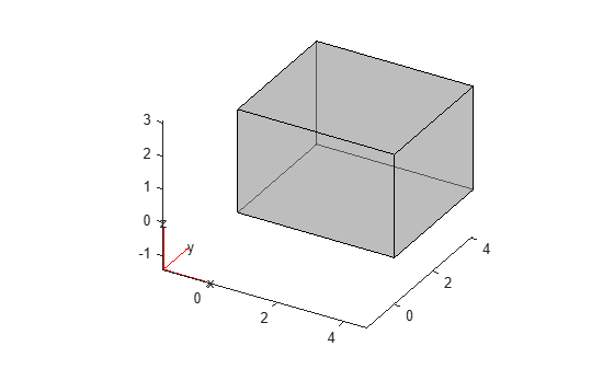
Create and plot the geometry of a shoebox room with the width, depth, and height specified in meters.

W = 4.7;
D = 4.1;
H = 3.1;
room = multicuboid(W,D,H);
room = translate(room,[W/2,D/2,0]);
pdegplot(room,FaceAlpha=0.5)

Assume that the room is highly reverberant with a near-zero absorption coefficient.

absrb = 3e-2;

Find the total absorption in the room.

A = absrb*(2*W*D+2*W*H+2*D*H);

Compute the reverberation time and the Schroeder frequency of the room.

V = W*D*H;
RT60 = 0.161*V/A

RT60 = 
3.4435

Find the Schroeder frequency of the room.

schroederFrequency = 2000*sqrt(RT60/V)

schroederFrequency = 
480.1838

Define the frequency interval over which to search for room modes.

frequencyRange = [20 schroederFrequency];

Convert the frequency range from hertz to radians per second.

w = frequencyRange*2*pi;

Specify Parameters of PDE Model

Create the PDE model and set its geometry to the empty rectangular room.

model = createpde;
model.Geometry = room;

The resonant frequencies of the room are the solutions of the Helmholtz equation ([3]):

$\Delta p+k^{2}p=0$,

where $p$ is the pressure, and $k$ is the wavenumber, defined as $k=\frac{w}{c_0},$ where w is the frequency (in radians/second) and $c_0$ is the speed of sound (meters/second). Since solving the Helmholtz equation is similar to solving the eigenvalue problem, the resulting k factors are referred to as eigenvalues, and the corresponding frequencies $f_k=\frac{c_0}{2\pi }k$ , at which the room resonates, are referred to as eigenfrequencies. The corresponding spatial pressure distributions $p_k\left(x,y,z\right)$are the room modes.

The PDE model solves eigenvalue equations of the following forms:

$-\nabla .\left(c\nabla p\right)+\text{a}p=\lambda \text{d}p$.

By comparing those equations to the Helmholtz equation, you get: $\lambda =w^2$, c = -1, a = 0, d = $\frac{-1}{c_0^2}$. Specify the coefficients of the PDE.

c0 = 343; % speed of sound (meters/second)
specifyCoefficients(model,d=-(1/c0).^2,c=-1,a=0,f=0,m=0);

For the room with rigid, perfectly reflecting surfaces, the boundary condition at the walls is the zero Neumann boundary condition ([3]) as $\frac{\delta p}{\delta n}=0$, where n is the direction normal to the boundary (the walls, floor and ceiling). The PDE model uses the zero Neumann boundary condition by default.

Generate Mesh and Solve Model

Typically, the mesh element size must be 0.1 of the wavelength$\lambda =\frac{c_0}{f}$ of the highest frequency of interest, where $f$ is the frequency, in hertz. In this example, to speed up computations, use the mesh element size equal to 0.2 of the wavelength. Generate a mesh for the room geometry assuming the highest frequency is 150 Hz.

FTarget = 150;
hmax = 0.2*c0/FTarget;
generateMesh(model,Hmax=hmax);

Find the eigenfrequencies recalling that $\lambda =w^2$.

results = solvepdeeig(model,w.^2);

Find the resonant frequencies of the room, in hertz.

f = sqrt(results.Eigenvalues)/(2*pi);

Compare Simulation Eigenfrequencies and Modes of Rectangular Room to Theoretical Results

Compare Eigenfrequencies

According to [3], you can compute the theoretical eigenfrequencies of a rectangular room with rigid boundaries as follows:

$F_{n_x,n_y,n_z}=\frac{c_0}{2}\sqrt{{\left(\frac{n_x}{W}\right)}^2+{\left(\frac{n_y}{D}\right)}^2+{\left(\frac{n_z}{H}\right)}^2}$,

where $n_x,n_y,n_z$ are nonnegative integers. Compute the first few theoretical eigenfrequencies.

nx = 0:7;
ny = 0:7;
nz = 0:7;
[A,B,C] = meshgrid(nx,ny,nz);
FTheory = (c0/2)*sqrt((A/W).^2+(B/D).^2+(C/H).^2);

Discard the zero-frequency mode (also called the cavity mode in [4]).

FTheory = FTheory(:);
FTheory = FTheory(2:end);
NxVect = A(:); 
NxVect = NxVect(2:end);
NyVect = B(:); 
NyVect = NyVect(2:end);
NzVect = C(:); 
NzVect = NzVect(2:end);

Sort the theoretical frequencies in ascending order.

[FTheory,ind] = sort(FTheory(:));
NxVect = NxVect(ind);
NyVect = NyVect(ind);
NzVect = NzVect(ind);
[~,idx2] = sort(f);

To compare simulation eigenfrequencies to theoretical results create a table that shows them side-by-side. Restrict the results to the first 50 frequencies.

N = 50;
T = table(NxVect(1:N),NyVect(1:N),NzVect(1:N), ...
          FTheory(1:N),f(1:N),idx2(1:N));
T.Properties.VariableNames = ...
    ["Nx","Ny","Nz","EigenFrequency_Theory", ...
     "EigenFrequency_Sim","Sim Index"];
disp(T)

    Nx    Ny    Nz    EigenFrequency_Theory    EigenFrequency_Sim    Sim Index
    __    __    __    _____________________    __________________    _________

    1     0     0            36.489                  36.489              1    
    0     1     0            41.829                  41.829              2    
    0     0     1            55.323                  55.324              3    
    1     1     0            55.508                  55.509              4    
    1     0     1            66.273                  66.275              5    
    0     1     1            69.356                  69.359              6    
    2     0     0            72.979                  72.983              7    
    1     1     1            78.369                  78.375              8    
    0     2     0            83.659                  83.666              9    
    2     1     0            84.116                  84.124             10    
    1     2     0             91.27                  91.281             11    
    2     0     1            91.578                  91.591             12    
    0     2     1             100.3                  100.32             13    
    2     1     1            100.68                   100.7             14    
    1     2     1            106.73                  106.75             15    
    3     0     0            109.47                   109.5             16    
    0     0     2            110.65                  110.68             17    
    2     2     0            111.02                  111.05             18    
    1     0     2            116.51                  116.55             19    
    3     1     0            117.19                  117.23             20    
    0     1     2            118.29                  118.33             21    
    3     0     1            122.65                  122.71             22    
    1     1     2            123.79                  123.84             23    
    2     2     1            124.04                  124.09             24    
    0     3     0            125.49                  125.54             25    
    3     1     1            129.59                  129.66             26    
    1     3     0            130.69                  130.75             27    
    2     0     2            132.55                  132.62             28    
    0     3     1            137.14                  137.23             29    
    3     2     0            137.78                  137.87             30    
    0     2     2            138.71                  138.81             31    
    2     1     2            138.99                  139.09             32    
    1     3     1            141.91                  142.01             33    
    1     2     2            143.43                  143.54             34    
    2     3     0            145.17                  145.27             35    
    4     0     0            145.96                  146.08             36    
    3     2     1            148.47                   148.6             37    
    4     1     0            151.83                  151.98             38    
    2     3     1            155.35                   155.5             39    
    3     0     2            155.65                  155.82             40    
    4     0     1            156.09                  156.26             41    
    2     2     2            156.74                  156.92             42    
    3     1     2            161.17                  161.37             43    
    4     1     1             161.6                  161.79             44    
    0     0     3            165.97                   166.2             45    
    3     3     0            166.52                  166.75             46    
    0     3     2             167.3                  167.53             47    
    0     4     0            167.32                  167.55             48    
    4     2     0            168.23                  168.47             49    
    1     0     3            169.93                  170.19             50    

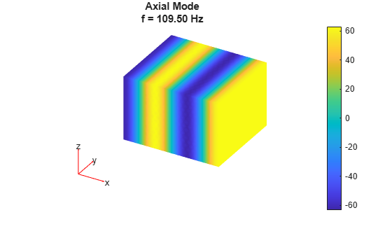
Plot and Compare Axial Mode

Solutions where only one of $n_x,n_y,n_z$ is nonzero correspond to waves where propagation is parallel to one of the room edges. The corresponding vibration pattern is called an axial mode. Extract an axial mode solution from the table and plot the corresponding solution.

TT=T(T.Nx==3 & T.Ny==0 & T.Nz==0,:);
N = TT.("Sim Index");

pdeplot3D(model.Mesh, ...
Colormap=results.Eigenvectors(:,N));
title(["Axial Mode", ...
sprintf("f = %0.2f Hz",TT.EigenFrequency_Sim)])
colormap parula

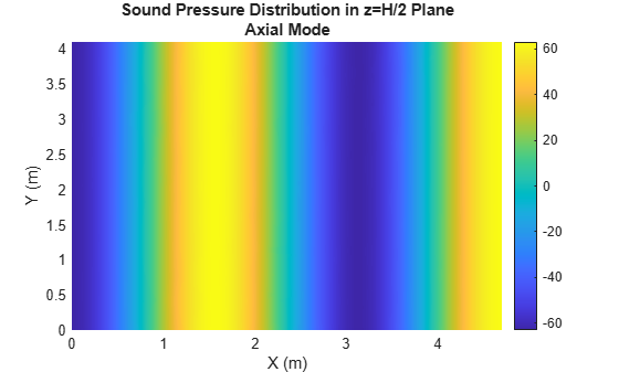
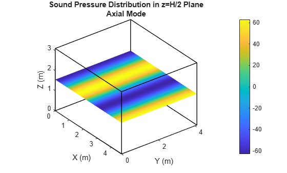
Plot the mode for the horizontal plane defined by z = H/2. First, interpolate the results for this plane.

xx = 0:W/200:W;
yy = 0:D/200:D;
[XX,YY] = meshgrid(xx,yy);
ZZ = (H/2)*ones(size(XX));

Vq = interpolateSolution(results,XX,YY,ZZ,N);

Plot the axial room mode in the horizontal plane.

Vq = reshape(Vq,size(XX));
figure
surface(xx,yy,Vq)
shading interp
colorbar
xlabel("X (m)")
ylabel("Y (m)")
axis tight
title(["Sound Pressure Distribution in z=H/2 Plane", ...
"Axial Mode"])

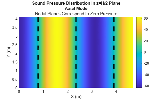
Now, compare the resulting axial mode to the theoretical axial mode. According to [3], you can compute the theoretical room modes as follows:

$p_{\text{nx},\text{ny},\text{nz}}=C.\cos \left(\frac{n_x\pi x}{W}\right).\cos \left(\frac{n_y\pi y}{D}\right).\cos \left(\frac{n_z\pi z}{H}\right)$,

where C is a constant. Thus, the axial mode is:

$p_{3,0,0}=C.\cos \left(\frac{3\pi x}{W}\right)$.

Note that the mode is equal to zero for odd multiples of W/6. The values of x for which the mode is equal to zero and which fall inside the room are W/6, W/2, and 5W/6. The planes perpendicular to the x-axis and defined by those values are called nodal planes. Sound pressure vanishes for all points in these planes.

Overlay the nodal planes on the plot. They correspond to simulated results of zero-pressure.

hold on
nx = TT.Nx;
X = (1:2:5)*W/(2*nx);
for index=1:numel(X)
    [mux,ax]=meshgrid(X(index),yy);
plot3(mux,ax,repmat(X(index),1,numel(yy)), ...
LineWidth=3,Color="k",LineStyle="--")
end
subtitle("Nodal Planes Correspond to Zero Pressure")
hold off

Plot the plane pressure distribution in 3-D.

visualizeModeInPlane3D(W,D,H,XX,YY,ZZ,Vq)
title(["Sound Pressure Distribution in z=H/2 Plane",...)
"Axial Mode"])

Visualize and Compare Tangential Mode

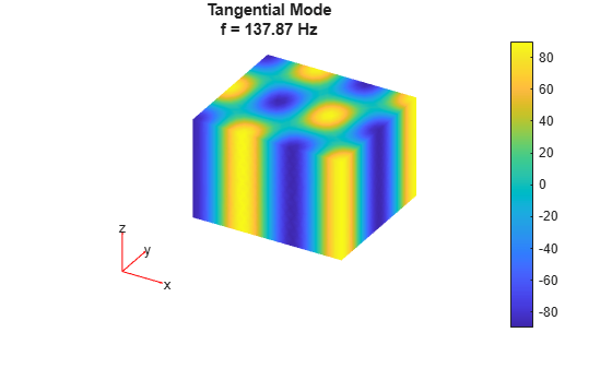
Solutions where only one of $n_x,n_y,n_z$ is zero correspond to waves where propagation is perpendicular to an axis, that is, parallel to all planes which are perpendicular to that axis. The corresponding vibration pattern is called a tangential mode. Extract a tangential mode solution from the table.

TT=T(T.Nx==3 & T.Ny==2 & T.Nz==0,:);
N = TT.("Sim Index");

Plot the corresponding mode.

pdeplot3D(model.Mesh, ...
Colormap=results.Eigenvectors(:,N));
title(["Tangential Mode", ...
sprintf("f = %0.2f Hz", ...
sqrt(results.Eigenvalues(N))/(2*pi))])
colormap parula

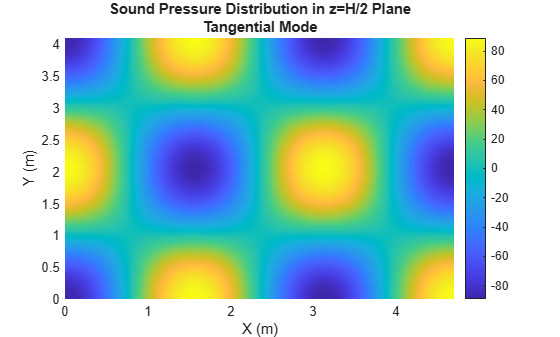
Now plot the solution for the horizontal plane z = H/2. First, interpolate the results for this plane.

xx = 0:W/200:W;
yy = 0:D/200:D;
[XX,YY] = meshgrid(xx,yy);
ZZ = H/2*ones(size(XX));

Vq = interpolateSolution(results,XX,YY,ZZ,N);

Plot the results.

Vq = reshape(Vq,size(XX));
figure
surface(xx,yy,Vq)
shading interp
colorbar
xlabel("X (m)")
ylabel("Y (m)")
axis tight
title(["Sound Pressure Distribution in z=H/2 Plane", ...
"Tangential Mode"])

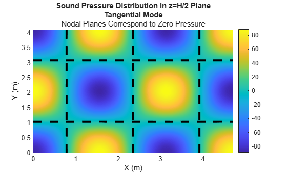
The theoretical room mode is:

$p_{3,2,0}=C.\cos \left(\frac{3\pi x}{W}\right).\cos \left(\frac{2\pi y}{D}\right)$.

The mode is equal to zero when x is equal to odd multiples of W/6 or when y is equal to odd multiples of D/4. Overlay the nodal planes that fall inside the room on the plot. These planes correspond to the simulated areas of zero-pressure.

hold on
nx = TT.Nx;
ny = TT.Ny;
X = (1:2:5)*W/(2*nx);
Y = (1:2:3)*D/(2*ny);

for index=1:numel(X)
    [mux,ax]=meshgrid(X(index),yy);
plot3(mux,ax,repmat(X(index),1,numel(yy)), ...
LineWidth=3,Color="k",LineStyle="--")
end
for index=1:numel(Y)
    [ax,muy]=meshgrid(xx,Y(index));
plot3(ax,muy,repmat(Y(index),1,numel(xx)), ...
LineWidth=3,Color="k",LineStyle="--")
end
subtitle("Nodal Planes Correspond to Zero Pressure")
hold off

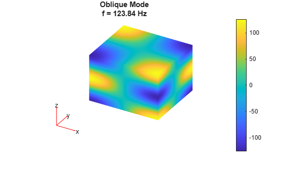
Plot and Compare Oblique Mode

Solutions where $n_x,n_y,n_z$ are nonzero correspond to waves where propagation involves all six surfaces and are called an oblique mode. Extract an oblique mode solution from the table.

TT=T(T.Nx==1 & T.Ny==1 & T.Nz==2,:);
N = TT.("Sim Index");

Plot the corresponding mode.

pdeplot3D(model.Mesh, ...
Colormap=results.Eigenvectors(:,N));
title(["Oblique Mode", ...
sprintf("f = %0.2f Hz", ...
sqrt(results.Eigenvalues(N))/(2*pi))])
colormap parula

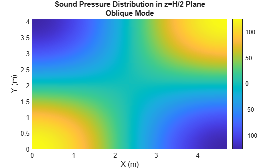
Now plot the solution for the horizontal plane z = H/2. First, interpolate the results for this plane.

xx = 0:W/200:W;
yy = 0:D/200:D;
[XX,YY] = meshgrid(xx,yy);
ZZ = H/2*ones(size(XX));

Vq = interpolateSolution(results,XX,YY,ZZ,N);
Vq = reshape(Vq,size(XX));

Plot the results.

Vq = reshape(Vq,size(XX));
figure
surface(xx,yy,Vq)
shading interp
colorbar
xlabel("X (m)")
ylabel("Y (m)")
axis tight
title(["Sound Pressure Distribution in z=H/2 Plane", ...
"Oblique Mode"])

Find Modes of Nonrectangular Room

Import and plot the geometry of a nonrectangular room.

g = importGeometry("customRoom.stl");
pdegplot(g)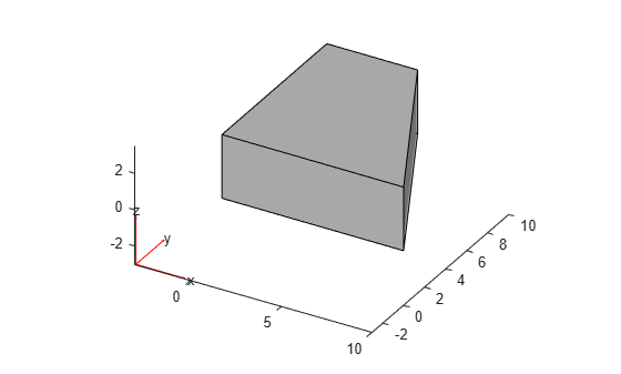

Set the geometry of the model to the nonrectangular room.

model.Geometry = g;

The Helmholtz equation that you solve to compute the eigenfrequencies does not depend on the room geometry. Therefore, you do not need to modify the PDE coefficients. Also, since the walls, floor, and ceiling of the room are rigid, the default zero Neumann boundary condition applies.

Because you modified the geometry, regenerate the mesh.

generateMesh(model,Hmax=hmax);

Solve for the eigenfrequencies and modes.

results = solvepdeeig(model,w.^2);

Extract the eigenfrequencies and display the first few values.

f = sqrt(results.Eigenvalues)/(2*pi);
f(1:10)

ans = 10×1

   21.6172
   30.1054
   35.2757
   38.5956
   42.7001
   49.0005
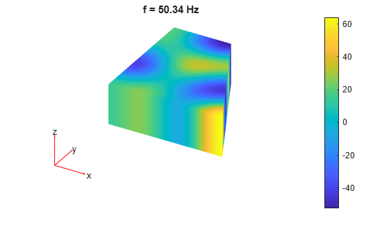
   50.3394
   51.6555
   52.1060
   53.5573

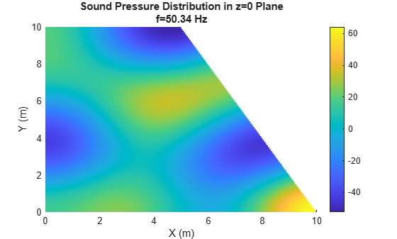
Plot the room mode for one eigenfrequency, for example, choose the seventh eigenfrequency.

figure
N = 7;
pdeplot3D(model.Mesh, ...
Colormap=results.Eigenvectors(:,N));
title(sprintf("f = %0.2f Hz", ...
sqrt(results.Eigenvalues(N))/(2*pi)))
colormap parula

Plot the solution for the horizontal plane (z=0). First, interpolate the results for this plane.

Lx = max(model.Geometry.Vertices(:,1));
xx = 0:Lx/200:Lx;
Ly = max(model.Geometry.Vertices(:,2));
yy = 0:Ly/200:Ly;
[XX,YY] = meshgrid(xx,yy);
ZZ = zeros(size(XX));

Vq = interpolateSolution(results,XX,YY,ZZ,N);
Vq = reshape(Vq,size(XX));

Plot the results.

Vq = reshape(Vq,size(XX));
figure
surface(xx,yy,Vq)
shading interp
colorbar
xlabel("X (m)")
ylabel("Y (m)")
axis tight
title(["Sound Pressure Distribution in z=0 Plane", ...
sprintf("f=%0.2f Hz",f(N))])

Helper Function

Visualize a room mode in a plane in 3-D.

function visualizeModeInPlane3D(L,W,H,XX,YY,ZZ,Vq)
% L: Room length
% W: Room width
% H: Room height
% XX: X mesh grid
% YY: Y mesh grid
% ZZ: Z mesh grid
% Vq: Output of interpolateSolution

% Outline the 3D room from (0,0,0) to (L,W,H)
V = [0 0 0;
    L 0 0;
    L W 0;
    0 W 0;
    0 0 H;
    L 0 H;
    L W H;
    0 W H];
E = [1 2;2 3;3 4;4 1; 5 6;6 7;7 8;8 5; 1 5;2 6;3 7;4 8];
figure;
hold on;
for e=1:size(E,1)
    plot3(V(E(e,:),1), V(E(e,:),2), V(E(e,:),3),"k-",LineWidth=1);
end

% Surface plot of the slice
surf(XX,YY,ZZ,Vq,EdgeColor="none");

shading interp;
colorbar;
xlabel("X (m)")
ylabel("Y (m)")
zlabel("Z (m)");
axis([0 L 0 W 0 H])
axis equal;

% Align the axes with pdeplot3D
view(3)
[caz,cel] = view;
view(caz-270,cel)

hold off
end

References

[1] The Schroeder Frequency: A Show and Tell, Part 1: https://www.soundandvision.com/content/schroeder-frequency-show-and-tell-part-1

[2] Reverbaration time and Sabine's Formula: https://www.acousticlab.com/en/reverberation-time-and-sabines-formula

[3] Kuttruff, Heinrich. Room Acoustics. Sixth edition, CRC Press, 2016.

[4] Jacobsen, Finn, and Peter Moller Juhl. Fundamentals of General Linear Acoustics. John Wiley & Sons Inc., 2013.