Speaker Identification Using Custom SincNet Layer and Deep Learning

This example uses:

In this example, you train three convolutional neural networks (CNNs) to perform speaker verification and then compare the performances of the architectures. The architectures of the three CNNs are all equivalent except for the first convolutional layer in each:

In the first architecture, the first convolutional layer is a "standard" convolutional layer, implemented using convolution2dLayer.
In the second architecture, the first convolutional layer is a constant sinc filterbank, implemented using a custom layer.
In the third architecture, the first convolutional layer is a trainable sinc filterbank, implemented using a custom layer. This architecture is referred to as SincNet [1].

[1] shows that replacing the standard convolutional layer with a filterbank layer leads to faster training convergence and higher accuracy. [1] also shows that making the parameters of the filter bank learnable yields additional performance gains.

Introduction

Speaker identification is a prominent research area with a variety of applications including forensics and biometric authentication. Many speaker identification systems depend on precomputed features such as i-vectors or MFCCs, which are then fed into machine learning or deep learning networks for classification. Other deep learning speech systems bypass the feature extraction stage and feed the audio signal directly to the network. In such end-to-end systems, the network directly learns low-level audio signal characteristics.

In this example, you first train a traditional end-to-end speaker identification CNN. The filters learned tend to have random shapes that do not correspond to perceptual evidence or knowledge of how the human ear works, especially in scenarios where the amount of training data is limited [1]. You then replace the first convolutional layer in the network with a custom sinc filterbank layer that introduces structure and constraints based on perceptual evidence. Finally, you train the SincNet architecture, which adds learnability to the sinc filterbank parameters.

The three neural network architectures explored in the example are summarized as follows:

Standard Convolutional Neural Network - The input waveform is directly connected to a randomly initialized convolutional layer which attempts to learn features and capture characteristics from the raw audio frames.
ConstantSincLayer - The input waveform is convolved with a set of fixed-width sinc functions (bandpass filters) equally spaced on the mel scale.
SincNetLayer - The input waveform is convolved with a set of sinc functions whose parameters are learned by the network. In the SincNet architecture, the network tunes parameters of the sinc functions while training.

This example defines and trains the three neural networks proposed above and evaluates their performance on the LibriSpeech Dataset [2].

Data Set

Download Dataset

In this example, you use a subset of the LibriSpeech Dataset [2]. The LibriSpeech Dataset is a large corpus of read English speech sampled at 16 kHz. The data is derived from audiobooks read from the LibriVox project.

dataFolder = tempdir;

dataset = fullfile(dataFolder,"LibriSpeech","train-clean-100");
if ~datasetExists(dataset)
    filename = "train-clean-100.tar.gz";
	url = "http://www.openSLR.org/resources/12/" + filename;
    gunzip(url,dataFolder);
    unzippedFile = fullfile(dataset,filename);
    untar(unzippedFile{1}(1:end-3),dataset);
end

Create an audioDatastore object to access the LibriSpeech audio data.

ads = audioDatastore(dataset,IncludeSubfolders=true);

Extract the speaker label from the file path.

ads.Labels = folders2labels(ads);

The full dev-train-100 dataset is around 6 GB of data. To run this example quickly, set speedupExample to true.

speedupExample = false;
if speedupExample
    allSpeakers = unique(ads.Labels);
    subsetSpeakers = allSpeakers(1:50);
    ads = subset(ads,ismember(ads.Labels,subsetSpeakers));
    ads.Labels = removecats(ads.Labels);
end
ads = splitEachLabel(ads,0.1);

Split the audio files into training and test data. 80% of the audio files are assigned to the training set and 20% are assigned to the test set.

[adsTrain,adsTest] = splitEachLabel(ads,0.8);

Sample Speech Signal

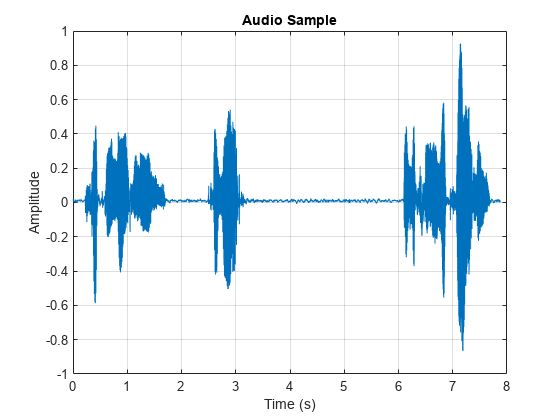
Plot one of the audio files and listen to it.

[audioIn,dsInfo] = read(adsTrain);
Fs = dsInfo.SampleRate;

sound(audioIn,Fs)

t = (1/Fs)*(0:length(audioIn)-1);

plot(t,audioIn)
title("Audio Sample")
xlabel("Time (s)")
ylabel("Amplitude")
grid on

Figure contains an axes object. The axes object with title Audio Sample, xlabel Time (s), ylabel Amplitude contains an object of type line.

Reset the training datastore.

reset(adsTrain)

Data Preprocessing

CNNs expect inputs to have consistent dimensions. You will preprocess the audio by removing regions of silence and then break the remaining speech into 200 ms frames with 40 ms overlap.

Set the parameters for preprocessing.

frameDuration = 200e-3;
overlapDuration = 40e-3;
frameLength = floor(Fs*frameDuration); 
overlapLength = round(Fs*overlapDuration);

Use the supporting function, preprocessAudioData, to preprocess the training and test data. Define a transform on the audio datastores to perform the preprocessing, then use readall to preprocess the entire datasets and place the preprocessed data into memory. If you have Parallel Computing Toolbox™, you can spread the computational load across workers. XTrain and XTest contain the train and test speech frames, respectively. TTrain and TTest contain the train and test labels, respectively.

pFlag = ~isempty(ver("parallel"));

adsTrainTransform = transform(adsTrain,@(x){preprocessAudioData(x,frameLength,overlapLength,Fs)});
XTrain = readall(adsTrainTransform,UseParallel=pFlag);

Starting parallel pool (parpool) using the 'Processes' profile ...
14-Nov-2023 09:44:47: Job Queued. Waiting for parallel pool job with ID 5 to start ...
14-Nov-2023 09:45:48: Job Queued. Waiting for parallel pool job with ID 5 to start ...
14-Nov-2023 09:46:49: Job Queued. Waiting for parallel pool job with ID 5 to start ...
14-Nov-2023 09:47:49: Job Queued. Waiting for parallel pool job with ID 5 to start ...
Connected to parallel pool with 6 workers.

Replicate the labels so that each 200 ms chunk has a corresponding label.

chunksPerFile = cellfun(@(x)size(x,4),XTrain);
TTrain = repelem(adsTrain.Labels,chunksPerFile,1);

Concatenate the training set into an array.

XTrain = cat(4,XTrain{:});

Perform the same preprocessing steps to the test set.

adsTestTransform = transform(adsTest,@(x){preprocessAudioData(x,frameLength,overlapLength,Fs)});
XTest = readall(adsTestTransform,UseParallel=true);
chunksPerFile = cellfun(@(x)size(x,4),XTest);
TTest = repelem(adsTest.Labels,chunksPerFile,1);
XTest = cat(4,XTest{:});

Standard CNN

Define Layers

The standard CNN is inspired by the neural network architecture in [1].

numFilters = 80;
filterLength = 251;
numSpeakers = numel(unique(removecats(ads.Labels)));

layers = [   

    imageInputLayer([1 frameLength 1])

    % First convolutional layer
    
    convolution2dLayer([1 filterLength],numFilters)
    batchNormalizationLayer
    leakyReluLayer(0.2)
    maxPooling2dLayer([1 3])
    
    % This layer is followed by 2 convolutional layers
    
    convolution2dLayer([1 5],60)
    batchNormalizationLayer
    leakyReluLayer(0.2)
    maxPooling2dLayer([1 3])
    
    convolution2dLayer([1 5],60)
    batchNormalizationLayer
    leakyReluLayer(0.2)
    maxPooling2dLayer([1 3])

    % This is followed by 3 fully-connected layers
    
    fullyConnectedLayer(256)
    batchNormalizationLayer
    leakyReluLayer(0.2)
    
    fullyConnectedLayer(256)
    batchNormalizationLayer
    leakyReluLayer(0.2)

    fullyConnectedLayer(256)
    batchNormalizationLayer
    leakyReluLayer(0.2)

    fullyConnectedLayer(numSpeakers)
    softmaxLayer];

Analyze the layers of the neural network using the analyzeNetwork function

analyzeNetwork(layers)

Train Network

Train the neural network for 15 epochs using adam optimization. Shuffle the training data before every epoch. The training options for the neural network are set using trainingOptions. Use the test data as the validation data to observe how the network performance improves as training progresses.

numEpochs = 15;
miniBatchSize = 128;
validationFrequency = floor(numel(TTrain)/miniBatchSize);

options = trainingOptions("adam", ...
    Shuffle="every-epoch", ...
    MiniBatchSize=miniBatchSize, ...
    Plots="training-progress", ...
    Verbose=false,MaxEpochs=numEpochs, ...
    ValidationData={XTest,categorical(TTest)}, ...
    ValidationFrequency=validationFrequency,...
    Metrics="accuracy");

To train the network, call trainnet.

[convNet,convNetInfo] = trainnet(XTrain,TTrain,layers,"crossentropy",options);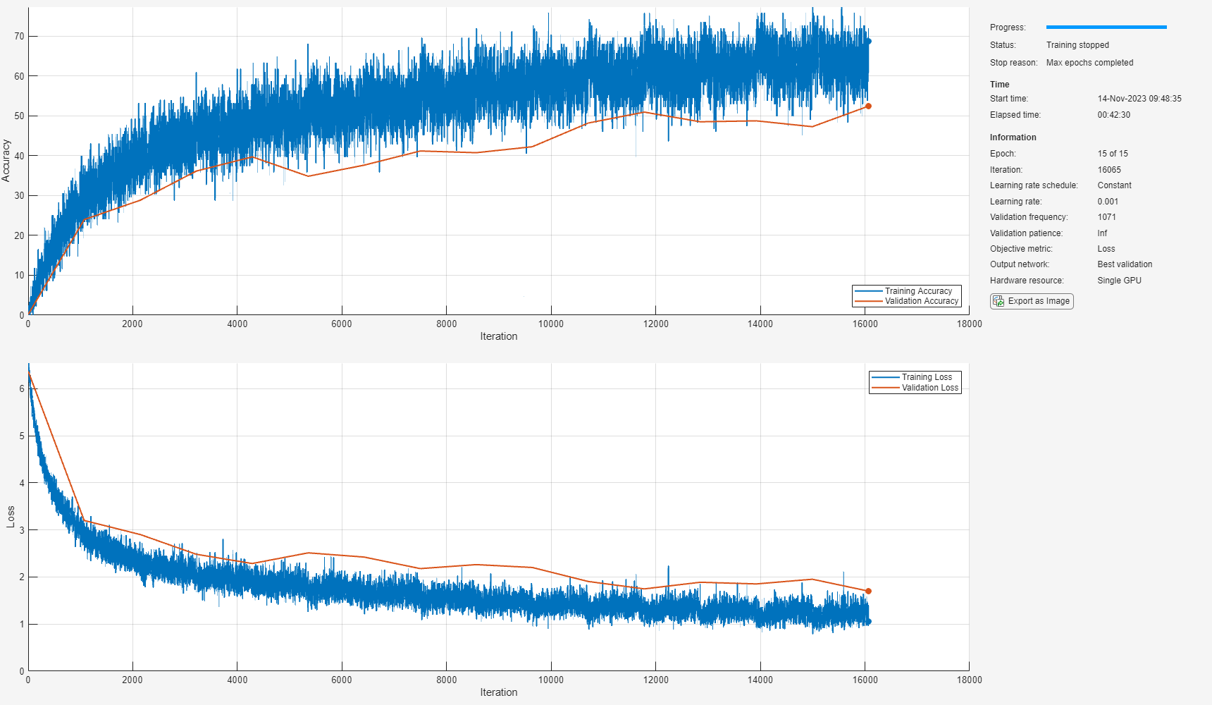

Recall that each signal is broken into short frames. There is a predicted speaker for each frame. You can achieve higher accuracy by combining all frame predictions into one signal prediction using a mode operation.

predictions = minibatchpredict(convNet,XTest);
labels = unique(ads.Labels);
predictions =  scores2label(predictions,labels);

ind = 1;
finalPredictions = repmat(TTrain(1),length(chunksPerFile),1);
for index=1:length(chunksPerFile)
    numS = chunksPerFile(index);
    finalPredictions(index) = mode(predictions(ind:ind+numS-1));
    ind = ind+numS;
end

standardNetAccuracy = sum(adsTest.Labels == finalPredictions)/numel(adsTest.Labels);
fprintf("Standard network accuracy: %f percent\n",100*standardNetAccuracy);

Standard network accuracy: 82.278481 percent

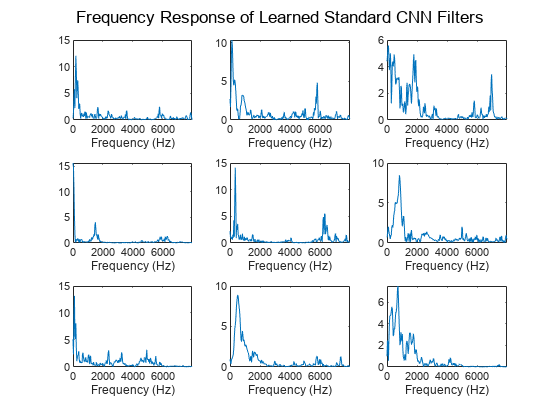
Inspect Frequency Response of First Convolutional Layer

Plot the magnitude frequency response of nine filters learned from the standard CNN network. The shape of these filters is not intuitive and does not correspond to perceptual knowledge. The next section explores the effect of using constrained filter shapes.

F = squeeze(convNet.Layers(2,1).Weights);
H = zeros(size(F));
Freq = zeros(size(F));

for ii = 1:size(F,2)
   [h,f] = freqz(F(:,ii),1,251,Fs);
    H(:,ii) = abs(h);
    Freq(:,ii) = f;
end
idx = linspace(1,size(F,2),9);
idx = round(idx);

figure
for jj = 1:9
   subplot(3,3,jj)
   plot(Freq(:,idx(jj)),H(:,idx(jj)))
   sgtitle("Frequency Response of Learned Standard CNN Filters")
   xlabel("Frequency (Hz)")
end

Constant Sinc Filterbank

In this section, you replace the first convolutional layer in the standard CNN with a constant sinc filterbank layer. The constant sinc filterbank layer convolves the input frames with a bank of fixed bandpass filters. The bandpass filters are a linear combination of two sinc filters in the time domain. The frequencies of the bandpass filters are spaced linearly on the mel scale.

Define Layers

The implementation for the constant sinc filterbank layer can be found in the constantSincLayer.m file (attached to this example). Define parameters for a ConstantSincLayer. Use 80 filters and a filter length of 251.

numFilters = 80;
filterLength = 251;
numChannels = 1;
name = "constant_sinc";

Change the first convolutional layer from the standard CNN to the ConstantSincLayer and keep the other layers unchanged.

cSL = constantSincLayer(numFilters,filterLength,Fs,numChannels,name)

cSL = 
  constantSincLayer with properties:

    Name: 'constant_sinc'

   Learnable Parameters
    No properties.

   State Parameters
    No properties.

  Show all properties

layers(2) = cSL;

Train Network

Train the network using the trainnet function. Use the same training options defined previously.

[constSincNet,constSincInfo] = trainnet(XTrain,TTrain,layers,"crossentropy",options);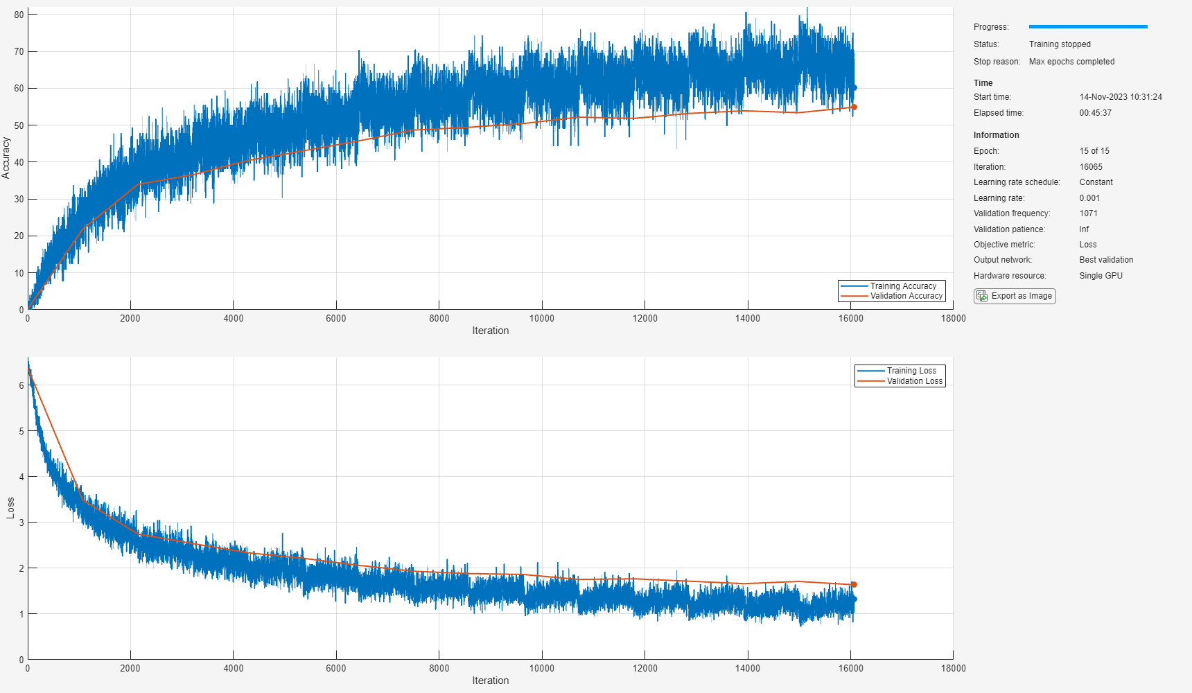

Similar to the regular network, combine individual frame predictions into a single prediction for each test audio signal.

constantSincNetAccuracy = getNetworkAccuracy(constSincNet,adsTest,XTest,labels,chunksPerFile);
fprintf("Constant SincNet network accuracy: %f percent\n",100*constantSincNetAccuracy);

Constant SincNet network accuracy: 87.341772 percent

Inspect Frequency Response of First Convolutional Layer

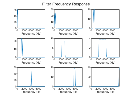
The plotNFilters method plots the magnitude frequency response of n filters with equally spaced filter indices. Plot the magnitude frequency response of nine filters in the ConstantSincLayer.

figure
n = 9;
plotNFilters(constSincNet.Layers(2),n)

SincNet

In this section, you use a trainable SincNet layer as the first convolutional layer in your network. The SincNet layer convolves the input frames with a bank of bandpass filters. The bandwidth and the initial frequencies of the SincNet filters are initialized as equally spaced in the mel scale. The SincNet layer attempts to learn better parameters for these bandpass filters within the neural network framework.

Define Layers

The implementation for the SincNet layer filterbank layer can be found in the sincNetLayer.m file (attached to this example). Define parameters for a SincNetLayer. Use 80 filters and a filter length of 251.

numFilters = 80;
filterLength = 251;
numChannels = 1; 
name = "sinc";

Replace the ConstantSincLayer from the previous network with the SincNetLayer. This new layer has two learnable parameters: FilterFrequencies and FilterBandwidths.

sNL = sincNetLayer(numFilters,filterLength,Fs,numChannels,name)

sNL = 
  sincNetLayer with properties:

                 Name: 'sinc'

   Learnable Parameters
    FilterFrequencies: [0.0019 0.0032 0.0047 0.0062 0.0078 0.0094 0.0111 0.0128 0.0145 0.0164 0.0183 0.0202 0.0222 0.0243 0.0264 0.0286 0.0309 0.0332 0.0356 0.0381 0.0407 0.0433 0.0460 0.0488 0.0517 0.0547 0.0578 0.0610 0.0643 0.0677 … ] (1×80 double)
     FilterBandwidths: [0.0028 0.0030 0.0031 0.0032 0.0033 0.0034 0.0035 0.0036 0.0037 0.0038 0.0039 0.0041 0.0042 0.0043 0.0045 0.0046 0.0047 0.0049 0.0051 0.0052 0.0054 0.0055 0.0057 0.0059 0.0061 0.0063 0.0065 0.0067 0.0069 0.0071 … ] (1×80 double)

   State Parameters
    No properties.

  Show all properties

layers(2) = sNL;

Train Network

Train the network using the trainnet function. Use the same training options defined previously.

[sincNet,sincNetInfo] = trainnet(XTrain,TTrain,layers,"crossentropy",options);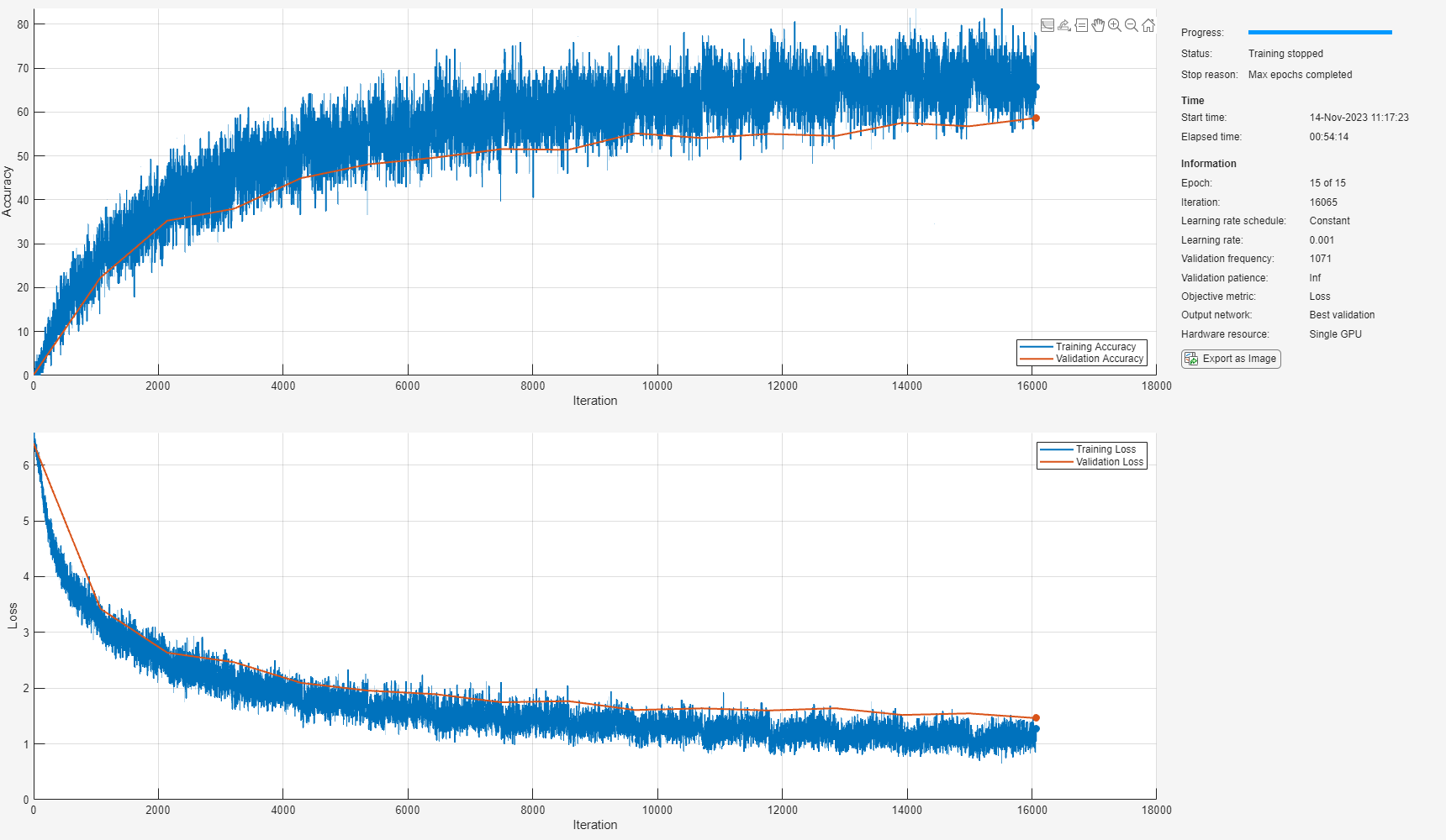

Similar to the regular network, combine individual frame predictions into a single prediction for each test audio signal.

sincNetNetAccuracy = getNetworkAccuracy(sincNet,adsTest,XTest,labels,chunksPerFile);
fprintf("SincNet network accuracy: %f percent\n",100*sincNetNetAccuracy);

SincNet network accuracy: 86.708861 percent

Inspect Frequency Response of First Convolutional Layer

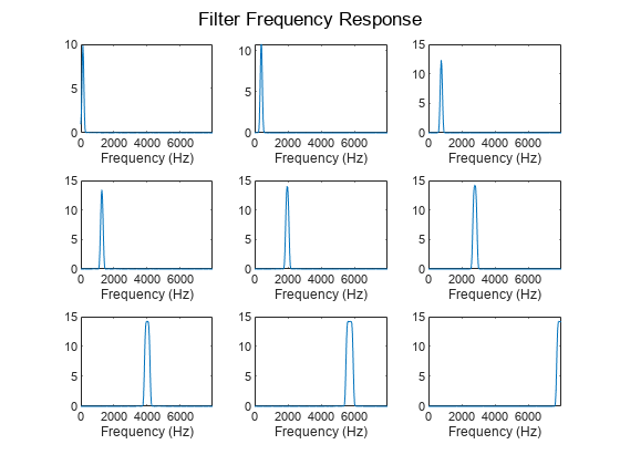
Use the plotNFilters method of SincNetLayer to visualize the magnitude frequency response of nine filters with equally spaced indices learned by SincNet.

figure
plotNFilters(sincNet.Layers(2),9)

Results Summary

Accuracy

The table summarizes the frame accuracy for all three neural networks.

NetworkType = ["Standard CNN";"Constant Sinc Layer";"SincNet Layer"];
Accuracy = [convNetInfo.ValidationHistory.Accuracy(end);constSincInfo.ValidationHistory.Accuracy(end);sincNetInfo.ValidationHistory.Accuracy(end)];
RefinedAccuracy = 100*[standardNetAccuracy;constantSincNetAccuracy;sincNetNetAccuracy];

resultsSummary = table(NetworkType,Accuracy,RefinedAccuracy)

resultsSummary=3×3 table
         NetworkType         Accuracy    RefinedAccuracy
    _____________________    ________    _______________

    "Standard CNN"            52.459         82.278     
    "Constant Sinc Layer"     54.885         87.342     
    "SincNet Layer"            58.63         86.709

Performance with Respect to Epochs

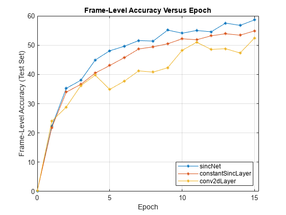
Plot the accuracy on the test set against the epoch number to see how well the networks learn as the number of epochs increase. SincNet outperforms the ConstantSincLayer network, especially during the early stages of training. This shows that updating the parameters of the bandpass filters within the neural network framework leads to faster convergence. This behavior is only observed when the dataset is large enough, so it might not be seen when speedupExample is set to true.

epoch = 0:numEpochs;

sinc_valAcc = sincNetInfo.ValidationHistory.Accuracy;
const_sinc_valAcc = constSincInfo.ValidationHistory.Accuracy;
conv_valAcc = convNetInfo.ValidationHistory.Accuracy;

figure
plot(epoch,sinc_valAcc,"-*",MarkerSize=4)
hold on
plot(epoch,const_sinc_valAcc,"-*",MarkerSize=4)
plot(epoch,conv_valAcc,"-*",MarkerSize=4)
ylabel("Frame-Level Accuracy (Test Set)")
xlabel("Epoch")
xlim([0 numEpochs+0.3])
title("Frame-Level Accuracy Versus Epoch")
legend("sincNet","constantSincLayer","conv2dLayer",Location="southeast")
grid on

Figure contains an axes object. The axes object with title Frame-Level Accuracy Versus Epoch, xlabel Epoch, ylabel Frame-Level Accuracy (Test Set) contains 3 objects of type line. These objects represent sincNet, constantSincLayer, conv2dLayer.

In the figure above, the final frame accuracy is a bit different from the frame accuracy that is computed in the last iteration. While training, the batch normalization layers perform normalization over mini-batches. However, at the end of training, the batch normalization layers normalize over the entire training data, which results in a slight change in performance.

Supporting Functions

function xp = preprocessAudioData(x,frameLength,overlapLength,Fs)

speechIdx = detectSpeech(x,Fs);
xp = zeros(1,frameLength,1,0);

for ii = 1:size(speechIdx,1)
    % Isolate speech segment
    audioChunk = x(speechIdx(ii,1):speechIdx(ii,2));

    % Split into 200 ms chunks
    audioChunk = buffer(audioChunk,frameLength,overlapLength);
    audioChunk = reshape(audioChunk,1,frameLength,1,size(audioChunk,2));

    % Concatenate with existing audio
    xp = cat(4,xp,audioChunk);
end
end


function accuracy = getNetworkAccuracy(net,adsTest,XTest,labels,numSegmentPerObservation)

predictions = minibatchpredict(net,XTest);
predictions =  scores2label(predictions,labels);

ind = 1;
finalPredictions = repmat(labels(1),length(numSegmentPerObservation),1);
for index=1:length(numSegmentPerObservation)
    numS = numSegmentPerObservation(index);
    finalPredictions(index) = mode(predictions(ind:ind+numS-1));
    ind = ind+numS;
end

accuracy = sum(adsTest.Labels == finalPredictions)/numel(adsTest.Labels);

end

References

[1] M. Ravanelli and Y. Bengio, "Speaker Recognition from Raw Waveform with SincNet," 2018 IEEE Spoken Language Technology Workshop (SLT), Athens, Greece, 2018, pp. 1021-1028, doi: 10.1109/SLT.2018.8639585.

[2] V. Panayotov, G. Chen, D. Povey and S. Khudanpur, "Librispeech: An ASR corpus based on public domain audio books," 2015 IEEE International Conference on Acoustics, Speech and Signal Processing (ICASSP), Brisbane, QLD, 2015, pp. 5206-5210, doi: 10.1109/ICASSP.2015.7178964