Train Voice Activity Detection in Noise Model Using Deep Learning
This example shows how to detect regions of speech in a low signal-to-noise environment using deep learning. You train a bidirectional long short-term memory (BiLSTM) network from scratch to perform voice activity detection (VAD) and compare that network to a pretrained deep learning-based VAD. To explore the model trained from scratch in this example, see Voice Activity Detection in Noise Using Deep Learning. To use an off-the-shelf deep learning-based VAD, see detectspeechnn.
Introduction
Voice activity detection is an essential component of many audio systems, such as automatic speech recognition, speaker recognition, and audio conferencing. Voice activity detection can be especially challenging in low signal-to-noise (SNR) situations, where speech is obstructed by noise.
For reproducibility, set the random seed to default.
rng defaultIn high SNR scenarios, traditional speech detection algorithms perform adequately. Read in an audio file that consists of words spoken with pauses between and listen to it.
fs = 16e3;
[speech,fileFs] = audioread("MaleVolumeUp-16-mono-6secs.ogg");
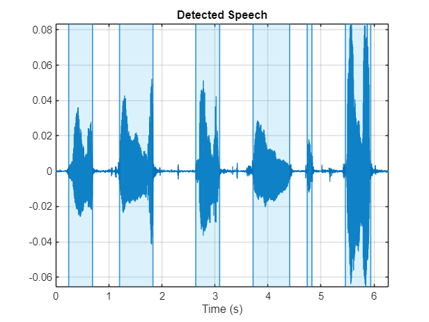
sound(speech,fs)Use the detectSpeech function to locate regions of speech. The detectSpeech function correctly identifies all regions of speech.
detectSpeech(speech,fs)
Load two noise signals and resample to the audio sample rate.
[noise200,fileFs200] = audioread("WashingMachine-16-8-mono-200secs.mp3");
[noise1000,fileFs1000] = audioread("WashingMachine-16-8-mono-1000secs.mp3");
noise200 = resample(noise200,fs,fileFs200);
noise1000 = resample(noise1000,fs,fileFs1000);
Use the supporting function mixSNR to corrupt the clean speech signal with washing machine noise at a desired SNR level in dB. Listen to the corrupted audio.
SNR = -10;
noisySpeech = mixSNR(speech,noise200,SNR);

sound(noisySpeech,fs)
-10;
noisySpeech = mixSNR(speech,noise200,SNR);
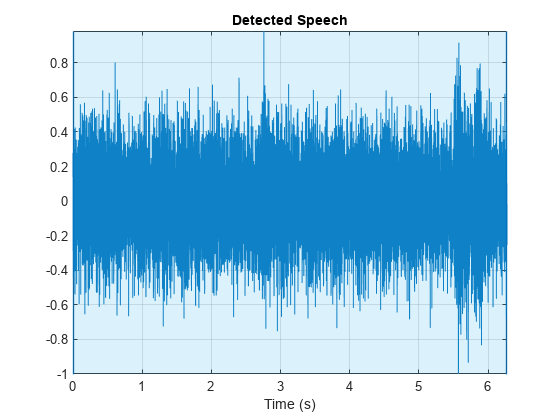
sound(noisySpeech,fs)Call detectSpeech on the noisy speech signal. The function fails to detect the speech regions given the very low SNR. The remainder of the example walks through training and evaluating deep learning-based VAD networks that can perform well under low SNR.
detectSpeech(noisySpeech,fs)
Download and Prepare Data
Download and extract the Google Speech Commands Dataset [1].
downloadFolder = matlab.internal.examples.downloadSupportFile("audio","google_speech.zip");
dataFolder = tempdir;
unzip(downloadFolder,dataFolder)
dataset = fullfile(dataFolder,"google_speech");
Create audioDatastore objects to point to the training and validation data sets.
adsTrain = audioDatastore(fullfile(dataset,"train"),IncludeSubfolders=true);
adsValidation = audioDatastore(fullfile(dataset,"validation"),IncludeSubfolders=true);
Construct Train and Validation Signals
The Google dataset consists of isolated words. Use the supporting function, constructSignal, to construct train and validation signals that consist of isolated words and regions of silence. The constructSignal function also returns ground truth binary masks indicating the regions of speech in the train and validation signals.
[audioTrain,TTrainPerSample] = constructSignal(adsTrain,fs,1000);
[audioValidation,TValidationPerSample] = constructSignal(adsValidation,fs,200);
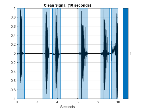
Listen to the first 10 seconds of the constructed signal. Use signalMask and plotsigroi to visualize the signal and ground truth binary mask.
duration =10; sound(audioTrain(1:duration*fs),fs) mask = signalMask(TTrainPerSample,SampleRate=fs); plotsigroi(mask,audioTrain,true) xlim([0,duration]) title("Clean Signal ("+duration+" seconds)")
Add Noise to Train and Validation Signals
Use the supporting function mixSNR to corrupt the train and validation signals with noise.
audioTrain = mixSNR(audioTrain,noise1000,SNR);
audioValidation = mixSNR(audioValidation,noise200,SNR);
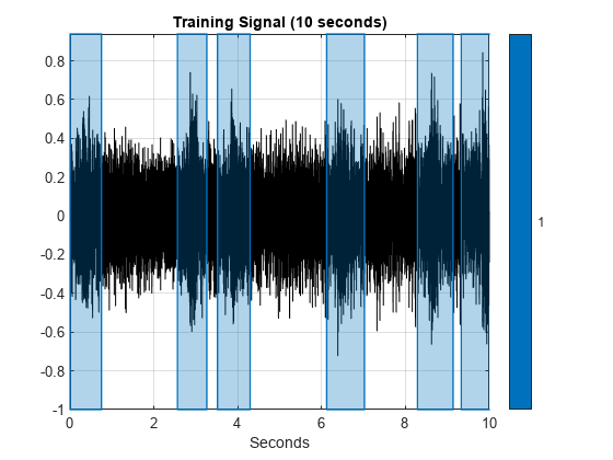
Listen to the first 10 seconds of the train signal and visualize the signal and mask.
sound(audioTrain(1:duration*fs),fs)

plotsigroi(mask,audioTrain,true)
xlim([0,duration])
title("Training Signal ("+duration+" seconds)")
Input Pipeline
Define an audioFeatureExtractor to extract the following spectral features: spectralCentroid, spectralCrest, spectralEntropy, spectralFlux, spectralKurtosis, spectralRolloffPoint, spectralSkewness, spectralSlope, and the periodicity feature harmonicRatio. Extract features using a 256-point Hann window with 50% overlap.
afe = audioFeatureExtractor(SampleRate=fs, ...
    Window=hann(256,"Periodic"), ...
    OverlapLength=128, ...
    ...
    spectralCentroid=true, ...
    spectralCrest=true, ...
    spectralEntropy=true, ...
    spectralFlux=true, ...
    spectralKurtosis=true, ...
    spectralRolloffPoint=true, ...
    spectralSkewness=true, ...
    spectralSlope=true, ...
    harmonicRatio=true);

featuresTrain = extract(afe,audioTrain);
Display the dimensions of the features matrix. The first dimension corresponds to the number of windows the signal was broken into (it depends on the signal length, window length, and overlap length). The second dimension is the number of features used in this example.
[numWindows,numFeatures] = size(featuresTrain)
numWindows =
124999
numFeatures =
9
In classification applications, it is a good practice to normalize all features to have zero mean and unity standard deviation.
Compute the mean and standard deviation for each coefficient, and use them to normalize the data.
M = mean(featuresTrain,1);
S = std(featuresTrain,[],1);
featuresTrain = (featuresTrain - M) ./ S;
Extract features from the validation signal using the same process.
XValidation = extract(afe,audioValidation);
XValidation = (XValidation - mean(XValidation,1)) ./ std(XValidation,[],1);
Each feature corresponds to 256 samples of data (the window length), sampled every 128 samples (the hop length). For each window, set the expected voice/no voice value to the mode of the baseline mask values corresponding to those 256 samples. Convert the voice/no voice mask to categorical.
windowLength = numel(afe.Window);
overlapLength = afe.OverlapLength;

TTrain = mode(buffer(TTrainPerSample,windowLength,overlapLength,"nodelay"),1);

TTrain = categorical(TTrain);
Do the same for the validation mask.
TValidation = mode(buffer(TValidationPerSample,windowLength,overlapLength,"nodelay"),1);

TValidation = categorical(TValidation);
Use the supporting function featureBuffer to split the training features and the mask into sequences with a duration approximately 8 seconds and a 75% overlap between consecutive sequences.
sequenceDuration =8; analysisHopLength = numel(afe.Window) - afe.OverlapLength; sequenceLength = round(sequenceDuration*fs/analysisHopLength); overlapPercent =
0.75; XTrain = featureBuffer(featuresTrain',sequenceLength,overlapPercent); TTrain = featureBuffer(TTrain,sequenceLength,overlapPercent);
Network Architecture
LSTM networks can learn long-term dependencies between time steps of sequence data. This example uses the bidirectional LSTM layer bilstmLayer (Deep Learning Toolbox) to look at the sequence in both forward and backward directions.
layers = [ ...
    sequenceInputLayer(afe.FeatureVectorLength)
    bilstmLayer(200,OutputMode="sequence")
    bilstmLayer(200,OutputMode="sequence")
    fullyConnectedLayer(2)
    softmaxLayer
    ];
Training Options
To define parameters for training, use trainingOptions (Deep Learning Toolbox). Use the Adam optimizer with a mini-batch size of 64 and a piecewise learn rate schedule.
maxEpochs =20; miniBatchSize =
64; options = trainingOptions("adam", ... MaxEpochs=maxEpochs, ... MiniBatchSize=miniBatchSize, ... Shuffle="every-epoch", ... Verbose=false, ... ValidationFrequency=floor(numel(XTrain)/miniBatchSize), ... ValidationData={XValidation.',TValidation}, ... Plots="training-progress", ... LearnRateSchedule="piecewise", ... Metrics = "Accuracy",... LearnRateDropFactor=0.1, ... LearnRateDropPeriod=5, ... OutputNetwork="best-validation-loss",... InputDataFormats = "CTB");
Train Network
To train the network, use trainnet.
speechDetectNet = trainnet(XTrain,TTrain,layers,"crossentropy" ,options);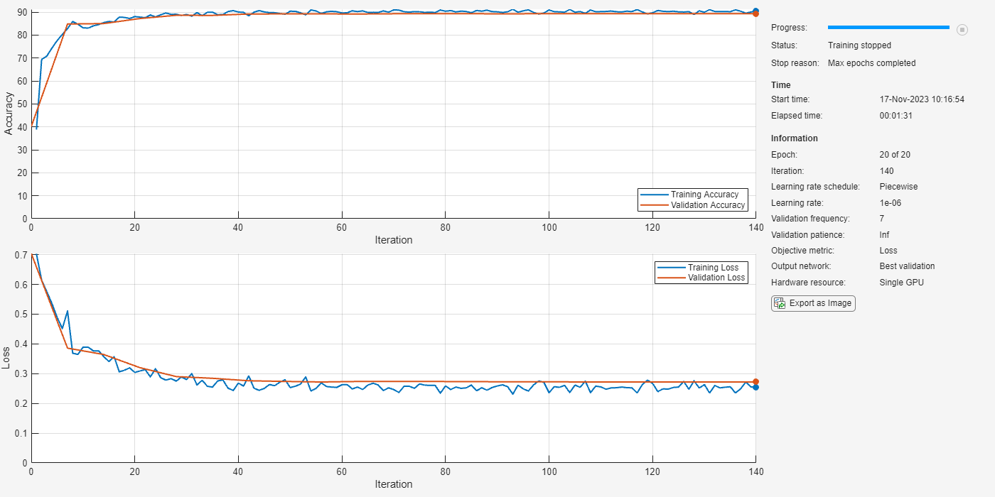
Evaluate Trained Network
Estimate voice activity in the validation signal using the trained network. Convert the estimated VAD mask from categorical to double, then replicate the window-based decisions to sample-based decisions.
YValidation = predict(speechDetectNet,XValidation);
YValidation = scores2label(YValidation,unique(TValidation));
YValidation = double(YValidation)-1;
wL = numel(afe.Window);
hL = wL - afe.OverlapLength;
YValidationPerSample = [repelem(YValidation(1),floor(wL/2 + hL/2),1);
    repelem(YValidation(2:end-1),hL,1);
    repelem(YValidation(end),ceil(wL/2 + hL/2),1)];
Calculate and plot the validation confusion matrix from the vectors of actual and estimated labels. Save the results for later analysis.
cc = confusionchart(TValidationPerSample,YValidationPerSample, ...
    title="speechDetect - Validation Confusion Chart", ...
    ColumnSummary="column-normalized",RowSummary="row-normalized");
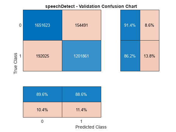
speechDetectResults = cc.NormalizedValues;
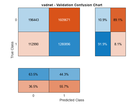
Evaluate Pretrained VAD Network
The vadnet network is a pretrained network for voice activity detection. You can use it with the vadnetPreprocess and vadnetPostprocess functions for applications such as transfer learning, or you can use detectspeechnn, which encapsulates vadnetPreprocess, vadnet, and vadnetPostprocess for inference-only applications. The vadnet network performs well under every-day adverse conditions, however it fails in the cases of extreme SNR, such as the -10 dB SNR used in this example. Also, vadnet was trained to detect regions of continuous speech (meaning several words in a row), not isolated words. In short, the pretrained vadnet fails for the validation signal in this example.
Load in the pretrained vadnet model.
net = audioPretrainedNetwork("vadnet");Extract features from the validation signal using the same input pipeline used to train the network.
XValidation = vadnetPreprocess(audioValidation,fs);
Predict the VAD mask.
y = predict(net,XValidation);
vadnet is a regression network and requires additional post-processing to determine decision boundaries. Use vadnetPostprocess to determine the boundaries of voice activity regions.
boundaries = vadnetPostprocess(audioValidation,16e3,y);
The vadnetPostprocess function returns the decisions as time boundaries. To convert the boundaries to a binary mask that corresponds to the original signal samples, use sigroi2binmask.
YValidationPerSample = double(sigroi2binmask(boundaries,size(audioValidation,1)));
To create a confusion chart to analyze the error, use confusionchart (Deep Learning Toolbox).
confusionchart(TValidationPerSample,YValidationPerSample, ...
    title="vadnet - Validation Confusion Chart", ...
    ColumnSummary="column-normalized",RowSummary="row-normalized");
Transfer Learning
Apply transfer learning to the pretrained vadnet to make use of both the pretrained weights and the network architecture.
Extract features from the audio.
featuresTrain = vadnetPreprocess(audioTrain,fs);
Buffer the ground truth mask so that decisions correspond to the analysis windows used in vadnetPreprocess.
windowLength = 400;
overlapLength = 240;
TTrainPerSamplePadded = [zeros(floor(windowLength/2),1);TTrainPerSample;zeros(ceil(windowLength/2),1)];
TTrain = mode(buffer(TTrainPerSamplePadded,windowLength,overlapLength,"nodelay"),1);
Buffer the validation mask.
TValidationPerSamplePadded = [zeros(floor(windowLength/2),1);TValidationPerSample;zeros(ceil(windowLength/2),1)];
TValidation = mode(buffer(TValidationPerSamplePadded,windowLength,overlapLength,"nodelay"),1);
Split the long training signal into overlapped sequences for training. Do the same for the ground-truth mask.
sequenceDuration =8; analysisHopLength = windowLength - overlapLength; sequenceLength = round(sequenceDuration*fs/analysisHopLength); overlapPercent =
0.75; XTrain = featureBuffer(featuresTrain,sequenceLength,overlapPercent); TTrain = featureBuffer(TTrain,sequenceLength,overlapPercent);
To define parameters for training, use trainingOptions (Deep Learning Toolbox).
miniBatchSize =12; maxEpochs =
9; options = trainingOptions("adam", ... InitialLearnRate=0.01, ... LearnRateSchedule="piecewise", ... LearnRateDropPeriod=3, ... MiniBatchSize=miniBatchSize, ... Shuffle="every-epoch", ... ValidationFrequency=floor(numel(XTrain)/miniBatchSize), ... ValidationData={XValidation,TValidation}, ... Verbose=false, ... Plots="training-progress", ... MaxEpochs=maxEpochs, ... OutputNetwork="best-validation-loss" ... );
To train the network, use trainnet.
noisyvadnet = trainnet(XTrain,TTrain,net,"mse",options);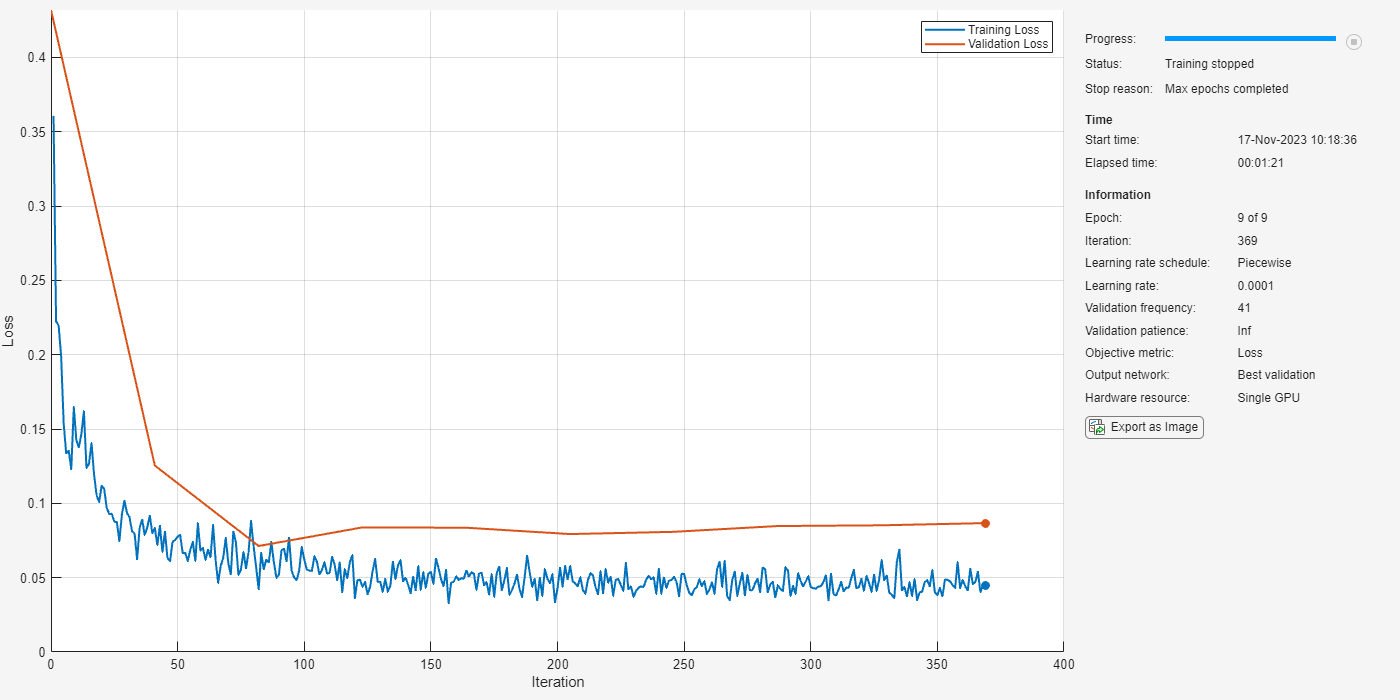
Estimate voice activity in the validation signal using the trained network. Postprocess the predictions using vadnetPostprocess, then convert the boundaries in time to a sample-based mask.
y = predict(noisyvadnet,gpuArray(XValidation));
boundaries = vadnetPostprocess(audioValidation,fs,y);
YValidationPerSample = double(sigroi2binmask(boundaries,size(audioValidation,1)));
Calculate and plot the validation confusion matrix from the vectors of actual and estimated labels. Save the results for later analysis.
cc = confusionchart(TValidationPerSample,YValidationPerSample, ...
    title="noisyvadnet - Validation Confusion Chart", ...
    ColumnSummary="column-normalized",RowSummary="row-normalized");
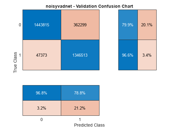
noisyvadnetResults = cc.NormalizedValues;
Compare Networks
There are several considerations when choosing a network, such as size, inference speed, error, and streaming capabilities.
Streaming
The speechDetectNet trained from scratch in this example is well-suited for streaming inference because its BiLSTM layers retain state between calls. See Voice Activity Detection in Noise Using Deep Learning for an example of using speechDetect for streaming voice activity detection.
The vadnet architecture consists of convolutional, recurrent, and fully-connected layers, and is not well-suited for low-latency streaming. See the vadnet documentation for an example of streaming VAD detection using vadnet.
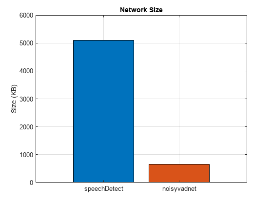
Network Size
Compare the network sizes.
networks = ["speechDetect","noisyvadnet"];
b = bar(reordercats(categorical(networks),networks),[whos("speechDetectNet").bytes/1024,whos("noisyvadnet").bytes/1024]);
title("Network Size")
ylabel("Size (KB)")
grid on
b.FaceColor = "flat";
b.CData(2,:) = [0.8500 0.3250 0.0980];
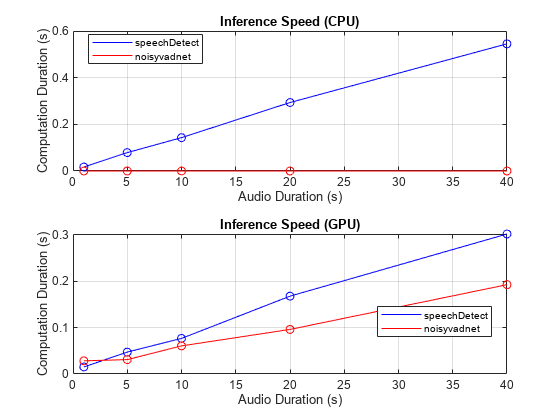
Network Inference Speed
Compare the network inference speeds. The simple speechDetect architecture has faster inference speed on both the CPU and the GPU for short durations (approximately 8 second chunks or less). For longer durations, speechDetect is faster than noisyvadnet on the GPU and slower on the CPU.
durationsToTest = [1,5,10,20,40];
environment = ["CPU","GPU"];

speechDetectSpeed = zeros(numel(durationsToTest),numel(environment));
noisyvadnetSpeed = zeros(numel(durationsToTest),numel(environment));
for jj = 1:numel(environment)
    for ii = 1:numel(durationsToTest)
        idx = 1:durationsToTest(ii)*fs;
        speechDetectFeatures = extract(afe,audioValidation(idx))';
        vadnetFeatures = vadnetPreprocess(audioValidation(idx),fs);

        switch environment(jj)
            case "CPU"
                speechDetectSpeed(ii,1) = timeit(@()predict(speechDetectNet,speechDetectFeatures.'),1);
                noisyvadnetSpeed(ii,1) = timeit(@()predict(noisyvadnet,vadnetFeatures),1);
            case "GPU"
                speechDetectSpeed(ii,2) = gputimeit(@()predict(speechDetectNet,gpuArray(speechDetectFeatures.')),1);
                noisyvadnetSpeed(ii,2) = gputimeit(@()predict(noisyvadnet,gpuArray(vadnetFeatures)),1);
        end
    end
end

tiledlayout(2,1)
for ii = 1:numel(environment)
    nexttile
    plot(durationsToTest,speechDetectSpeed(:,ii),"b-", ...
        durationsToTest,noisyvadnetSpeed(:,ii),"r-", ...
        durationsToTest,speechDetectSpeed(:,ii),"bo", ...
        durationsToTest,noisyvadnetSpeed(:,ii),"ro")
    legend(["speechDetect","noisyvadnet"],Location="best")
    grid on
    xlabel("Audio Duration (s)")
    ylabel("Computation Duration (s)")
    title("Inference Speed ("+environment(ii)+")")
end
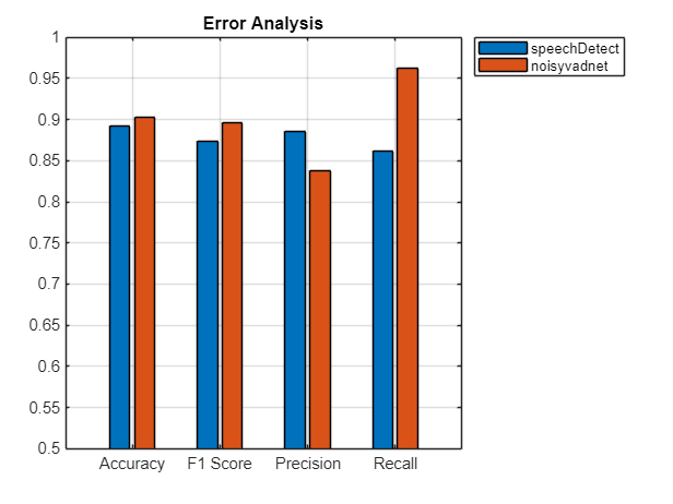
Network Error
Use the previously calculated confusion charts to display common statistics for error analysis. Accuracy, recall, precision, and f1 score are all derived from the confusion matrices previously plotted.
Accuracy is defined as the ratio of correctly predicted observations to the total observations. It is the most intuitive metric but can be misleading for imbalanced data sets. For example, if speech is only present in 5% of the audio, then classifying all audio as non-speech would result in 95 % accuracy.
Recall, also called sensitivity, is the ratio of correctly predicted positive observations to all observations that belong to the positive class. Recall answers the question: Of all speech regions, how many were correctly classified? A low recall indicates that regions of speech were misclassified as regions of nonspeech.
Precision is the ratio of correctly predicted positive observations to the total predicted positive observations. Precision answers the question: Of all the observations the network classified as speech, how many were actually speech? A low precision indicates that regions of nonspeech were misclassified as regions of speech.
F1 score is the harmonic mean of the precision and recall: it accounts for both false positives and false negatives.
The true measure of a network depends on your application. In real-world situations, a cost function is usually optimized which weights the costs of false positives and false negatives.
TP = speechDetectResults(2,2);
TN = speechDetectResults(1,1);
FP = speechDetectResults(1,2);
FN = speechDetectResults(2,1);
speechDetectAccuracy = (TP+TN)/(TP+TN+FP+FN);
speechDetectRecall = TP/(TP+FN);
speechDetectPrecision = TP/(TP+FP);
speechDetectF1Score = 2*(speechDetectRecall*speechDetectPrecision)/(speechDetectRecall+speechDetectPrecision);

TP = noisyvadnetResults(2,2);
TN = noisyvadnetResults(1,1);
FP = noisyvadnetResults(1,2);
FN = noisyvadnetResults(2,1);
noisyvadnetAccuracy = (TP+TN)/(TP+TN+FP+FN);
noisyvadnetRecall = TP/(TP+FN);
noisyvadnetPrecision = TP/(TP+FP);
noisyvadnetF1Score = 2*(noisyvadnetRecall*noisyvadnetPrecision)/(noisyvadnetRecall+noisyvadnetPrecision);

figure
bar(categorical(["Accuracy","Recall","Precision","F1 Score"]), ...
    [speechDetectAccuracy,noisyvadnetAccuracy; ...
    speechDetectRecall,noisyvadnetRecall; ...
    speechDetectPrecision,noisyvadnetPrecision; ...
    speechDetectF1Score,noisyvadnetF1Score]);
title("Error Analysis")
legend("speechDetect","noisyvadnet",Location="bestoutside")
ylim([0.5,1])
grid on
Supporting Functions
Convert Feature Vectors to Sequences
function sequences = featureBuffer(features,featureVectorsPerSequence,overlapPercent)
% y = featureBuffer(x,sequenceLength,overlapPercent) buffers a sequence of
% feature vectors, x, into sequences of length sequenceLength overlapped by
% overlapPercent. The sequences output are returns in a cell array for
% consumption by trainnet.

featureVectorOverlap = round(overlapPercent*featureVectorsPerSequence);
hopLength = featureVectorsPerSequence - featureVectorOverlap;

N = floor((size(features,2) - featureVectorsPerSequence)/hopLength) + 1;
sequences = cell(N,1);

idx = 1;
for jj = 1:N
    sequences{jj} = features(:,idx:idx + featureVectorsPerSequence - 1);
    idx = idx + hopLength;
end

end
Mix SNR
function [noisySignal,requestedNoise] = mixSNR(signal,noise,ratio)
% [noisySignal,requestedNoise] = mixSNR(signal,noise,ratio) returns a noisy
% version of the signal, noisySignal. The noisy signal has been mixed with
% noise at the specified ratio in dB.

numSamples = size(signal,1);

% Convert noise to mono
noise = mean(noise,2);

% Trim or expand noise to match signal size
if size(noise,1)>=numSamples
    % Choose a random starting index such that you still have numSamples
    % after indexing the noise.
    start = randi(size(noise,1) - numSamples + 1);
    noise = noise(start:start+numSamples-1);
else
    numReps = ceil(numSamples/size(noise,1));
    temp = repmat(noise,numReps,1);
    start = randi(size(temp,1) - numSamples - 1);
    noise = temp(start:start+numSamples-1);
end

signalNorm = norm(signal);
noiseNorm = norm(noise);

goalNoiseNorm = signalNorm/(10^(ratio/20));
factor = goalNoiseNorm/noiseNorm;

requestedNoise = noise.*factor;
noisySignal = signal + requestedNoise;

noisySignal = noisySignal./max(abs(noisySignal));
end
Construct Signal
function [audio,mask] = constructSignal(ds,fs,duration)
% [audio,mask] = constructSignal(ds,fs,duration) constructs an audio signal
% of the specified duration by concatenating samples from the
% audioDatastore ds with random duration of silence between.

win = hamming(50e-3*fs,"periodic");

% Create a 1000-second training signal by combining multiple speech files
% from the training data set. Use detectSpeech to remove unwanted portions
% of each file. Insert a random period of silence between speech segments.
% Preallocate the training signal.
N = duration*fs;
audio = zeros(N,1);

% Preallocate the voice activity training mask. Values of 1 in the mask
% correspond to samples located in areas with voice activity. Values of 0
% correspond to areas with no voice activity.
mask = zeros(N,1);

% Specify a maximum silence segment duration of 2 seconds.
maxSilenceSegment = 2;

% Construct the training signal by calling read on the datastore in a loop.
numSamples = 1;
while numSamples < N
    data = read(ds);
    data = data ./ max(abs(data)); % Scale amplitude

    % Determine regions of speech
    idx = detectSpeech(data,fs,Window=win);

    % If a region of speech is detected
    if ~isempty(idx)

        % Extend the indices by five frames
        idx(1,1) = max(1,idx(1,1) - 5*numel(win));
        idx(1,2) = min(length(data),idx(1,2) + 5*numel(win));

        % Isolate the speech
        data = data(idx(1,1):idx(1,2));

        % Write speech segment to training signal
        audio(numSamples:numSamples+numel(data)-1) = data;

        % Set VAD baseline
        mask(numSamples:numSamples+numel(data)-1) = true;

        % Random silence period
        numSilenceSamples = randi(maxSilenceSegment*fs,1,1);
        numSamples = numSamples + numel(data) + numSilenceSamples;
    end
end
audio = audio(1:N);
mask = mask(1:N);
end
References
[1] Warden P. "Speech Commands: A public dataset for single-word speech recognition", 2017. Available from https://storage.googleapis.com/download.tensorflow.org/data/speech_commands_v0.01.tar.gz. Copyright Google 2017. The Speech Commands Dataset is licensed under the Creative Commons Attribution 4.0 license