resample

Resample uniform or nonuniform data to new fixed rate

Syntax

y = resample(x,p,q)

y = resample(x,p,q,n)

y = resample(x,p,q,n,beta)

y = resample(x,p,q,b)

yTT = resample(xTT,p,q,___)

y = resample(x,tx)

y = resample(x,tx,fs)

y = resample(x,tx,fs,p,q)

y = resample(x,tx,___,method)

[y,ty] = resample(x,tx,___)

yTT = resample(xTT,___)

[y,b] = resample(x,p,q,___)

[y,ty,b] = resample(x,tx,___)

[yTT,b] = resample(xTT,___)

[___] = resample(___,Dimension=dim)

Description

y = resample(x,p,q) resamples the input sequence, x, at p/q times the original sample rate. resample applies an FIR Antialiasing Lowpass Filter to x and compensates for the delay introduced by the filter. The function operates along the first array dimension with size greater than 1.

y = resample(x,p,q,n) uses an antialiasing filter of order 2 × n × max(p,q).

y = resample(x,p,q,n,beta) specifies the shape parameter of the Kaiser window used to design the lowpass filter.

y = resample(x,p,q,b) filters x using the filter coefficients specified in b.

yTT = resample(xTT,p,q,___) resamples the uniformly sampled data in the MATLAB^® timetable xTT at p/q times the original sample rate and returns a timetable yTT. You can specify additional arguments n, beta, or b.

y = resample(x,tx) resamples the values, x, of a signal sampled at the instants specified in vector tx. The function interpolates x linearly onto a vector of uniformly spaced instants with the same endpoints and number of samples as tx. NaNs are treated as missing data and are ignored.

y = resample(x,tx,fs) uses a polyphase antialiasing filter to resample the signal at the uniform sample rate specified in fs.

y = resample(x,tx,fs,p,q) interpolates the input signal to an intermediate uniform grid with a sample spacing of (p/q)/fs. The function then filters the result to upsample it by p and downsample it by q, resulting in a final sample rate of fs. For best results, ensure that fs × q/p is at least twice as large as the highest frequency component of x.

y = resample(x,tx,___,method) specifies the interpolation method along with any of the arguments from previous syntaxes in this group. The interpolation method can be "linear", "pchip", or "spline".

[y,ty] = resample(x,tx,___) returns in ty the instants that correspond to the resampled signal.

yTT = resample(xTT,___) resamples the nonuniformly sampled data in xTT and returns uniformly sampled data. yTT has the same endpoints and number of samples as xTT. You can specify the same argument options available for input x,tx.

[y,b] = resample(x,p,q,___) also returns the coefficients of the filter applied to x during the resampling.

[y,ty,b] = resample(x,tx,___) returns in b the coefficients of the antialiasing filter.

[yTT,b] = resample(xTT,___) resamples the timetable data in xTT and also returns the coefficients of the antialiasing filter in b.

[___] = resample(___,Dimension=dim) resamples the input along dimension dim. (since R2020b)

Examples

Resample Linear Sequence

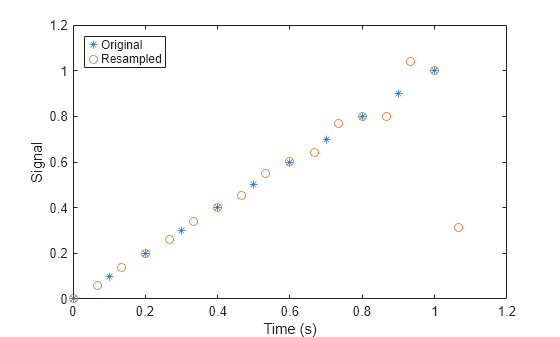
Resample a simple linear sequence at 3/2 the original rate of 10 Hz. Plot the original and resampled signals on the same figure.

fs = 10;
t1 = 0:1/fs:1;
x = t1;
y = resample(x,3,2);
t2 = (0:(length(y)-1))*2/(3*fs);

plot(t1,x,'*',t2,y,'o')
xlabel('Time (s)')
ylabel('Signal')
legend('Original','Resampled', ...
    'Location','NorthWest')

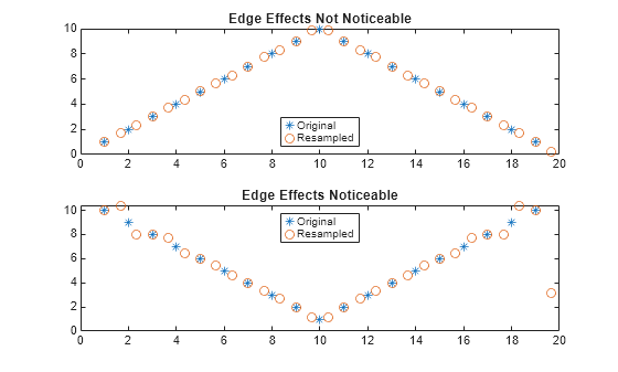
When filtering, resample assumes that the input sequence, x, is zero before and after the samples it is given. Large deviations from zero at the endpoints of x can result in unexpected values for y.

Show these deviations by resampling a triangular sequence and a vertically shifted version of the sequence with nonzero endpoints.

x = [1:10 9:-1:1;
    10:-1:1 2:10]';
y = resample(x,3,2);

subplot(2,1,1)
plot(1:19,x(:,1),'*',(0:28)*2/3 + 1,y(:,1),'o')
title('Edge Effects Not Noticeable')
legend('Original','Resampled', ...
    'Location','South')

subplot(2,1,2)
plot(1:19,x(:,2),'*',(0:28)*2/3 + 1,y(:,2),'o')
title('Edge Effects Noticeable')
legend('Original','Resampled', ...
    'Location','North')

Resample Using Kaiser Window

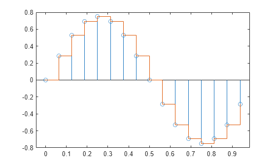
Construct a sinusoidal signal. Specify a sample rate such that 16 samples correspond to exactly one signal period. Draw a stem plot of the signal. Overlay a stairstep graph for sample-and-hold visualization.

fs = 16;
t = 0:1/fs:1-1/fs;

x = 0.75*sin(2*pi*t);

stem(t,x)
hold on
stairs(t,x)
hold off

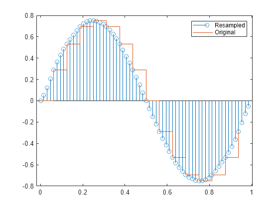
Use resample to upsample the signal by a factor of four. Use the default settings. Plot the result alongside the original signal.

ups = 4;
dns = 1;

fu = fs*ups;
tu = 0:1/fu:1-1/fu;

y = resample(x,ups,dns);

stem(tu,y)
hold on
stairs(t,x)
hold off
legend("Resampled","Original")

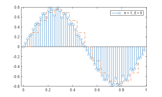
Repeat the calculation. Specify n = 1 so that the antialiasing filter is of order $$2\times 1\times 4=8$$. Specify a shape parameter $$\beta =0$$ for the Kaiser window. Output the filter as well as the resampled signal.

n = 1;
beta = 0;

[y,b] = resample(x,ups,dns,n,beta);

fo = filtord(b)

fo = 
8

stem(tu,y)
hold on
stairs(t,x,"--")
hold off
legend("n = 1, \beta = 0")

The resampled signal shows aliasing effects that result from the relatively wide mainlobe and low sidelobe attenuation of the window.

Increase n to 5 and leave $$\beta =0$$. Verify that the filter is of order 40. Plot the resampled signal.

n = 5;

[y,b] = resample(x,ups,dns,n,beta);

fo = filtord(b)

fo = 
40

stem(tu,y)
hold on
stairs(t,x,"--")
hold off
legend("n = 5, \beta = 0")

The longer window has a narrower mainlobe and attenuates aliasing effects better. It also attenuates the signal.

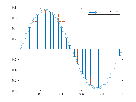
Leave the filter order at $$2\times 5\times 4=40$$ and increase the shape parameter to $$\beta =20$$.

beta = 20;

y = resample(x,ups,dns,n,beta);

stem(tu,y)
hold on
stairs(t,x,"--")
hold off
legend("n = 5, \beta = 20")

The high sidelobe attenuation results in good resampling.

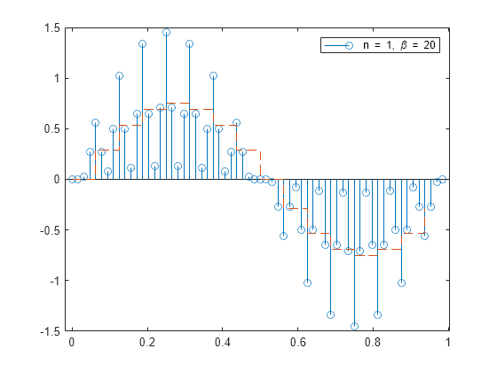
Decrease the filter order back to $$2\times 1\times 4=8$$ and leave $$\beta =20$$.

n = 1;

[y,b] = resample(x,ups,dns,n,beta);

stem(tu,y)
hold on
stairs(t,x,"--")
hold off
legend("n = 1, \beta = 20")

The wider mainlobe generates considerable artifacts upon resampling.

Resample a Sinusoid

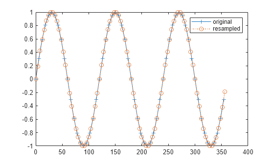
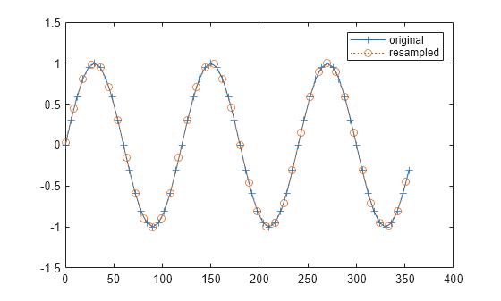
Generate 60 samples of a sinusoid and resample it at 3/2 the original rate. Display the original and resampled signals.

tx = 0:6:360-3;
x = sin(2*pi*tx/120);

ty = 0:4:360-2;
[y,by] = resample(x,3,2);

plot(tx,x,'+-',ty,y,'o:')
legend('original','resampled')

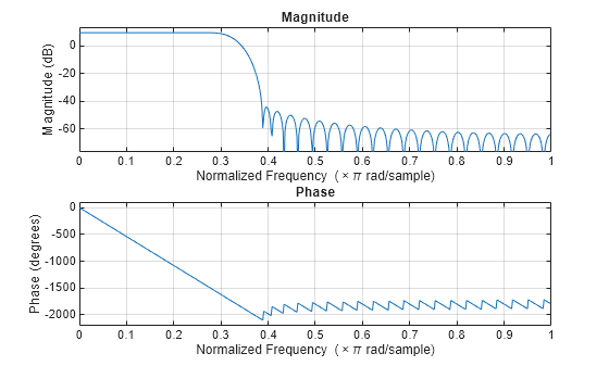
Plot the frequency response of the anti-aliasing filter.

freqz(by)

Resample the signal at 2/3 the original rate. Display the original signal and its resampling.

tz = 0:9:360-9;
[z,bz] = resample(x,2,3);

plot(tx,x,'+-',tz,z,'o:')
legend('original','resampled')

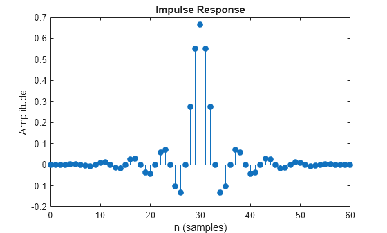
Plot the impulse response of the new lowpass filter.

impz(bz)

Resample Data in Timetable

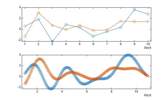
Create two vectors of ten randomly generated numbers. Assume one number for each vector was recorded daily for a total of ten days. Store the data in a MATLAB timetable.

a = randn(10,1);
b = randn(10,1);

t = days(1:10);

xTT = timetable(t',[a b]);

Use the resample function to increase the sample rate from once daily to once hourly. Plot both data sets.

yTT = resample(xTT,24,1);

subplot(2,1,1)
plot(xTT.Time,xTT.Var1,'-o')
subplot(2,1,2)
plot(yTT.Time,yTT.Var1,'-o')

Resample a Nonuniformly Sampled Data Set

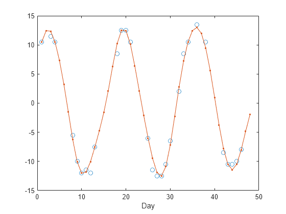
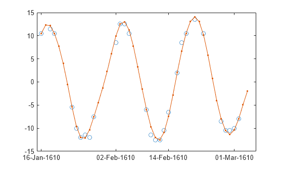
Use the data recorded by Galileo Galilei in 1610 to determine the orbital period of Callisto, the outermost of Jupiter's four largest satellites.

Galileo observed the satellites' motion for six weeks, starting on 15 January. The observations have several gaps because Jupiter was not visible on cloudy nights. Generate a datetime array of observation times.

t = [0 2 3 7 8 9 10 11 12 17 18 19 20 24 25 26 27 28 29 31 32 33 35 37 ...
    41 42 43 44 45]'+1;

yg = [10.5 11.5 10.5 -5.5 -10.0 -12.0 -11.5 -12.0 -7.5 8.5 12.5 12.5 ...
    10.5 -6.0 -11.5 -12.5 -12.5 -10.5 -6.5 2.0 8.5 10.5 13.5 10.5 -8.5 ...
    -10.5 -10.5 -10.0 -8.0]';

obsv = datetime(1610,1,15+t);

Resample the data onto a regular grid using a sample rate of one observation per day. Use a moderate upsampling factor of 3 to avoid overfitting.

fs = 1;

[y,ty] = resample(yg,t,fs,3,1);

Plot the data and the resampled signal.

plot(t,yg,'o',ty,y,'.-')
xlabel('Day')

Repeat the procedure using spline interpolation and displaying the observation dates. Express the sample rate in inverse days.

fs = 1/86400;

[ys,tys] = resample(yg,obsv,fs,3,1,'spline');

plot(t,yg,'o')
hold on
plot(ys,'.-')
hold off

ax = gca;
ax.XTick = t(1:9:end);
ax.XTickLabel = char(obsv(1:9:end));

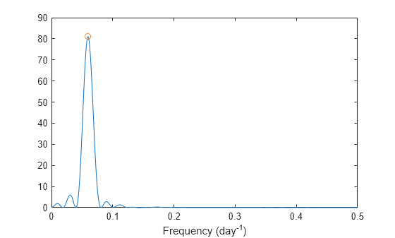
Compute the periodogram power spectrum estimate of the uniformly spaced, linearly interpolated data. Choose a DFT length of 1024. The signal peaks at the inverse of the orbital period.

[pxx,f] = periodogram(ys,[],1024,1,'power');
[pk,i0] = max(pxx);

f0 = f(i0);
T0 = 1/f0

T0 = 
16.7869

plot(f,pxx,f0,pk,'o')
xlabel('Frequency (day^{-1})')

Resample Nonuniformly Sampled Data in Timetable

A person recorded their weight in pounds most days of the leap year 2012. They entered missing samples as NaN. Load the data and store the measurements in a MATLAB timetable. Specify the row times using a datetime vector and remove the missing samples.

load weight2012.dat

rowTimes = datetime(2012,1,1:366)';
wt = weight2012(:,2);
xTT = timetable(rowTimes,wt);
xTT(isnan(wt),:) = [];

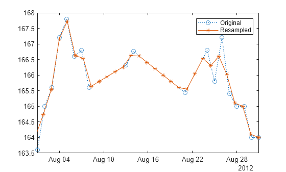
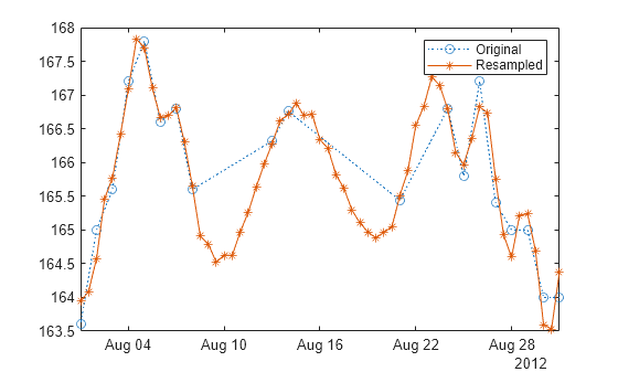
Resample the data. The result is a timetable containing uniformly sampled data with the same endpoints and number of samples as wt.

yTT = resample(xTT);

Plot both the original and the resampled data for comparison. Adjust the x-axis limits to display only the measurements in the month of August.

plot(xTT.rowTimes,xTT.wt,":o",yTT.Time,yTT.wt,"-*")
aug = datetime([2012 08 01;2012 08 31]); 
xlim(aug)
legend(["Original" "Resampled"])

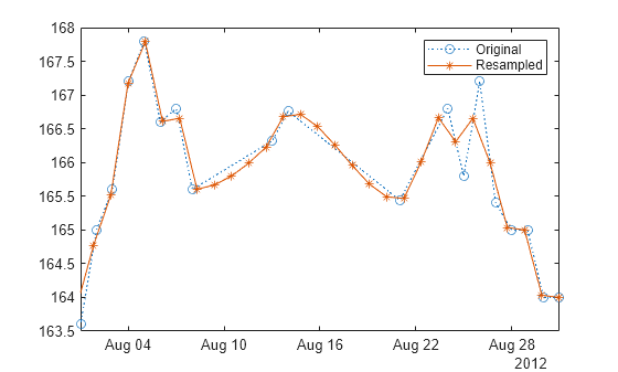
Resample the data again using cubic interpolation.

yTTs = resample(xTT,"pchip");

plot(xTT.rowTimes,xTT.wt,":o",yTTs.Time,yTTs.wt,"-*")
xlim(aug)
legend(["Original" "Resampled"])

Now increase the sample rate to two measurements per day and use spline interpolation. Plot the result.

fs = 1/86400;
yTTf = resample(xTT,2*fs,"spline");

plot(xTT.rowTimes,xTT.wt,":o",yTTf.Time,yTTf.wt,'-*')
xlim(aug)
legend(["Original" "Resampled"])

Resample Multichannel Signal

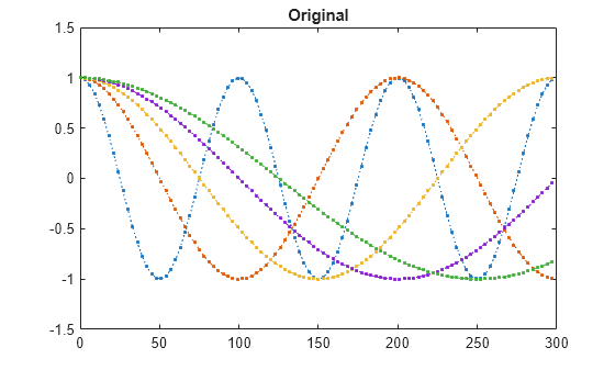
Generate a five-channel, 100-sample sinusoidal signal. Time increases across the columns and frequency increases down the rows. Plot the signal.

p = 3;
q = 2;

tx = 0:p:300-p;

x = cos(2*pi*tx./(1:5)'/100);

plot(tx,x,'.:')
title('Original')
ylim([-1.5 1.5])

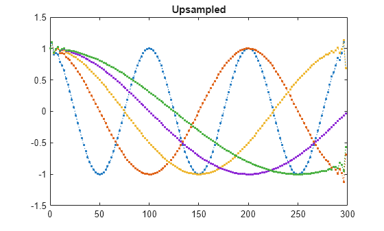
Upsample the sinusoid by 3/2 along its second dimension. Overlay the resampled signal on the plot.

ty = 0:q:300-q;

y = resample(x,p,q,'Dimension',2);

plot(ty,y,'.:')
title('Upsampled')

Reshape the resampled signal so that time runs along a third dimension.

y = permute(y,[1 3 2]);
size(y)

ans = 1×3

     5     1   150

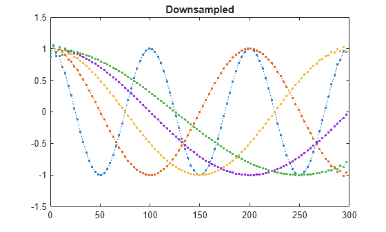
Downsample the signal back to its original rate and plot it.

z = resample(y,q,p,'Dimension',3);

plot(tx,squeeze(z),'.:')
title('Downsampled')

Input Arguments

x — Input signal

vector | matrix | N-D array

Input signal, specified as a vector, matrix, or N-D array. x can contain NaNs when time information is provided. NaNs are treated as missing data and are excluded from the resampling.

Example: cos(pi/4*(0:159))+randn(1,160) is a single-channel row-vector signal.

Example: cos(pi./[4;2]*(0:159))'+randn(160,2) is a two-channel signal.

Data Types: single | double

p, q — Resampling factors

positive integers

Resampling factors, specified as positive integers.

Data Types: single | double

n — Neighbor term number

10 (default) | nonnegative integer

Neighbor term number, specified as a nonnegative integer. If n = 0, resample performs nearest-neighbor interpolation. The length of the antialiasing FIR filter is proportional to n. Larger values of n provide better accuracy at the expense of more computation time.

Data Types: single | double

beta — Shape parameter of Kaiser window

5 (default) | positive real scalar

Shape parameter of Kaiser window, specified as a positive real scalar. Increasing beta widens the mainlobe of the window used to design the antialiasing filter and decreases the amplitude of the window’s sidelobes.

Data Types: single | double

b — FIR filter coefficients

vector

FIR filter coefficients, specified as a vector. By default, resample designs the filter using firls with a Kaiser window. When compensating for the delay, resample assumes b has odd length and linear phase. See Antialiasing Lowpass Filter for more information.

Data Types: single | double

xTT — Input timetable

timetable

Input timetable with at least two rows, specified as a timetable. Each variable in xTT is treated as an independent signal. If a variable in the timetable is an N-D array, then resample operates along the first dimension.

Note

• RowTimes must be either a duration vector or a datetime object with unique and finite values. Nonfinite time values are treated as missing data and are ignored.

• If unsorted, resample sorts RowTimes in ascending order.

For more information, see timetable.

tx — Time instants

nonnegative real vector | datetime array

Time instants, specified as a nonnegative real vector or a datetime array. tx must increase monotonically but need not be uniformly spaced. tx can contain NaNs or NaTs. These values are treated as missing data and excluded from the resampling. tx is valid only for input x.

Data Types: single | double | datetime

fs — Sample rate

positive scalar

Sample rate, specified as a positive scalar. The sample rate is the number of samples per unit time. If the unit of time is seconds, then the sample rate is in Hz.

Data Types: single | double

method — Interpolation method

"linear" (default) | "pchip" | "spline"

Interpolation method, specified as one of "linear", "pchip", or "spline":

• "linear" — Linear interpolation.

• "pchip" — Shape-preserving piecewise cubic interpolation.

• "spline" — Spline interpolation using not-a-knot end conditions.

For more information, see the interp1 reference page.

Note

If x is not slowly varying, consider using interp1 with the "pchip" interpolation method.

dim — Dimension to operate along

positive integer scalar

Dimension to operate along, specified as a positive integer scalar. If dim is not specified, resample operates along the first array dimension with size greater than 1. If the input is a timetable, then dim must be 1.

Data Types: single | double

Output Arguments

y — Resampled signal

vector | matrix | N-D array

Resampled signal, returned as a vector, matrix, or N-D array. If x is of length N along dimension dim and you specify p and q, then y is of length ⌈N × p/q⌉ along dim.

b — FIR filter coefficients

vector

FIR filter coefficients, returned as a vector.

ty — Output instants

nonnegative real vector

Output instants, returned as a nonnegative real vector. ty applies only for input x.

yTT — Resampled timetable

timetable

Resampled timetable, returned as a timetable.

More About

Antialiasing Lowpass Filter

To resample a signal by a rational factor p/q, resample calls upfirdn, which conceptually performs these steps:

1. Insert zeros to upsample the signal by p.

2. Apply an FIR antialiasing filter to the upsampled signal.

3. Discard samples to downsample the filtered signal by q.

The ideal antialiasing filter has normalized cutoff frequency f_c = π/max(p,q) rad/sample and gain p. To approximate the antialiasing filter, resample uses the Kaiser window method.

• The filter order is 2 × n × max(p,q). The default value of n is 10.

• The Kaiser window has a shape parameter beta that controls the tradeoff between transition width and stopband attenuation. The default value of beta is 5.

• The filter coefficients are normalized to account for the processing gain of the window.

As an example, design an antialiasing filter to resample a signal to 3/2 times its original sample rate:

p = 3;
q = 2;
maxpq = max(p,q);

fc = 1/maxpq;
n = 10;
order = 2*n*maxpq;
beta = 5;

b = fir1(order,fc,kaiser(order+1,beta));
b = p*b/sum(b);

For more information, see Resample Uniformly Sampled Signals.

Tips

• Use the isregular function to determine if a timetable is uniformly sampled.

Algorithms

resample performs an FIR design using firls, normalizes the result to account for the processing gain of the window, and then implements a rate change using upfirdn.

Extended Capabilities

C/C++ Code Generation

Generate C and C++ code using MATLAB® Coder™.

Usage notes and limitations:

• The resample function does not support timetable inputs for code generation.

• To generate optimized code that uses SIMD intrinsics and runs on ARM^® Cortex^®-A 32-bit/64-bit processors, you must install Embedded Coder^® Support Package for AMD SoC Devices. The support package for Xilinx^® Zynq^® Platform includes the ARM cross-compiler toolchains and enables deployment on ARM Cortex-A processors. MATLAB Support Package for Raspberry Pi^® Hardware enables a direct deployment of optimized code on ARM devices. For an example, see Generate Optimized Code on Raspberry Pi Target. (since R2022b)

• For ARM architectures, the resample function does not support single-precision inputs.

GPU Code Generation

Generate CUDA® code for NVIDIA® GPUs using GPU Coder™.

Usage notes and limitations:

• timetable inputs are not supported for code generation.

GPU Arrays

Accelerate code by running on a graphics processing unit (GPU) using Parallel Computing Toolbox™.

The resample function supports GPU array input with these usage notes and limitations:

• The "pchip" interpolation method is not supported.

• Input timetable containing a gpuArray is not supported.

For more information, see Run MATLAB Functions on a GPU (Parallel Computing Toolbox).

Version History

Introduced before R2006a

R2024a: Use datetime arrays for C/C++ code generation

The resample function supports datetime arrays for code generation. You must have MATLAB Coder™ to use this functionality.

R2023a: Use single-precision data

The resample function supports single-precision inputs.

R2020b: Resample multidimensional arrays

The resample function has a dim argument that you can use to specify the dimension along which to operate. If you do not specify the dim argument, resample operates along the first array dimension with size greater than 1. The output has the same number of dimensions as the input.