samplealign
Align two data sets containing sequential observations by introducing gaps
Syntax
[
I
, J
]
= samplealign(X
, Y
)
[I
, J
]
= samplealign(X
, Y
,
...'Band', BandValue
, ...)
[I
, J
]
= samplealign(X
, Y
,
...'Width', WidthValue
, ...)
[I
, J
]
= samplealign(X
, Y
,
...'Gap', GapValue
, ...)
[I
, J
]
= samplealign(X
, Y
,
...'Quantile', QuantileValue
, ...)
[I
, J
]
= samplealign(X
, Y
,
...'Distance', DistanceValue
, ...)
[I
, J
]
= samplealign(X
, Y
,
...'Weights', WeightsValue
, ...)
[I
, J
]
= samplealign(X
, Y
,
...'ShowConstraints', ShowConstraintsValue
,
...)
[I
, J
]
= samplealign(X
, Y
,
...'ShowNetwork', ShowNetworkValue
, ...)
[I
, J
]
= samplealign(X
, Y
,
...'ShowAlignment', ShowAlignmentValue
,
...)
Input Arguments
X , Y | Matrices of data where rows correspond to observations or samples,
and columns correspond to features or dimensions. X and Y can
have a different number of rows, but they must have the same number
of columns. The first column is the reference dimension and must contain
unique values in ascending order. The reference dimension could contain
sample indices of the observations or a measurable value, such as
time. |
BandValue | Either of the following:
|
WidthValue | Either of the following:
|
GapValue | Any of the following:
|
QuantileValue | Scalar between 0 and 1 that
specifies the quantile value used to calculate the term QMS ,
which is used by the 'Gap' property to calculate
gap penalties. Default is 0.75 . |
DistanceValue | Function handle specified using
Default is the Euclidean distance between the pairs. Caution All columns in |
WeightsValue | Either of the following:
This property controls the inclusion/exclusion
of columns (features) or the emphasis of columns (features) when calculating
the distance score between observations that are potential matches,
that is, when using the Tip Using a numeric row vector for Note The weight values are not considered when using the |
ShowConstraintsValue | Controls the display of the search space constrained by the
specified 'Band' and 'Width'
input parameters, thereby giving an indication of the memory required
to run the algorithm with the specific 'Band' and 'Width' parameters
on your data sets. Choices are true or false (default). |
ShowNetworkValue | Controls the display of the dynamic programming network, the
match scores, the gap penalties, and the winning path. Choices are true or false (default). |
ShowAlignmentValue | Controls the display of the first and second columns of the X and Y data
sets in the abscissa and the ordinate respectively, of a two-dimensional
plot. Choices are true , false (default),
or an integer specifying a column of the X and Y data
sets to plot as the ordinate. |
Output Arguments
I | Column vector containing indices of rows (observations) in X that
match to a row (observation) in Y . Missing
indices indicate that row (observation) is matched to a gap. |
J | Column vector containing indices of rows (observations) in Y that
match to a row (observation) in X . Missing
indices indicate that row (observation) is matched to a gap. |
Description
[
aligns
the observations in two matrices of data, I
, J
]
= samplealign(X
, Y
)X
and Y
,
by introducing gaps. X
and Y
are
matrices of data where rows correspond to observations or samples,
and columns correspond to features or dimensions. X
and Y
can
have different number of rows, but must have the same number of columns.
The first column is the reference dimension and must contain unique
values in ascending order. The reference dimension could contain sample
indices of the observations or a measurable value, such as time. The samplealign
function
uses a dynamic programming algorithm to minimize the sum of positive
scores resulting from pairs of observations that are potential matches
and the penalties resulting from the insertion of gaps. Return values I
and J
are
column vectors containing indices that indicate the matches for each
row (observation) in X
and Y
respectively.
Tip
If you do not specify return values, samplealign
does
not run the dynamic programming algorithm. Running samplealign
without
return values, but setting the 'ShowConstraints'
, 'ShowNetwork'
,
or 'ShowAlignment'
property to true
,
lets you explore the constrained search space, the dynamic programming
network, or the aligned observations, without running into potential
memory problems.
[
calls I
, J
]
= samplealign(X
, Y
,
...'PropertyName
', PropertyValue
,
...)samplealign
with optional
properties that use property name/property value pairs. You can specify
one or more properties in any order. Each PropertyName
must
be enclosed in single quotation marks and is case insensitive. These
property name/property value pairs are as follows:
[
specifies
a maximum allowable distance between observations (along the reference
dimension only) in the two data sets, thus limiting the number of
potential matches between observations in the two data sets. If I
, J
]
= samplealign(X
, Y
,
...'Band', BandValue
, ...)S
is
the value in the reference dimension for a given observation (row)
in one data set, then that observation is matched only with observations
in the other data set whose values in the reference dimension fall
within S
± BandValue
.
Then, only these potential matches are passed to the algorithm for
further scoring. BandValue
can be a scalar
or a function specified using @(
,
where z
)z
is the mid-point between a given
observation in one data set and a given observation in the other data
set. Default BandValue
is Inf
.
This constraint reduces the time and memory complexity of the
algorithm from O(MN
) to O(sqrt(MN
)*K
),
where M
and N
are
the number of observations in X
and Y
respectively,
and K
is a small constant such that K
<<M
and K
<<N
.
Adjust BandValue
to the maximum expected
shift between the reference dimensions in the two data sets, that
is, between X
(:,1) and Y
(:,1).
[
limits
the number of potential matches between observations in two data sets;
that is, each observation in I
, J
]
= samplealign(X
, Y
,
...'Width', WidthValue
, ...)X
is scored
to the closest U
observations in Y
,
and each observation in Y
is scored to
the closest V
observations in X
.
Then, only these potential matches are passed to the algorithm for
further scoring. WidthValue
is either a
two-element vector, [U
, V
]
or a scalar that is used for both U
and V
.
Closeness is measured using only the first column (reference dimension)
in each data set. Default is Inf
if 'Band'
is
specified; otherwise default is 10
.
This constraint reduces the time and memory complexity of the
algorithm from O(MN
) to O(sqrt(MN
)*sqrt(UV
)),
where M
and N
are
the number of observations in X
and Y
respectively,
and U
and V
are
small such that U
<<M
and V
<<N
.
Note
If you specify both 'Band'
and 'Width'
,
only pairs of observations that meet both constraints are considered
potential matches and passed to the algorithm for scoring.
Tip
Specify 'Width'
when you do not have a good
estimate for the 'Band'
property. To get an indication
of the memory required to run the algorithm with specific 'Band'
and 'Width'
parameters
on your data sets, run samplealign
, but do not
specify return values and set 'ShowConstraints'
to true
.
[
specifies
the position-dependent terms for assigning gap penalties. I
, J
]
= samplealign(X
, Y
,
...'Gap', GapValue
, ...)
GapValue
is any of the following:
Cell array, {
G
,H
}, whereG
is either a scalar or a function handle specified using@(
, andX
)H
is either a scalar or a function handle specified using@(
. The functionsY
)@(
andX
)@(
must calculate the penalty for each observation (row) when it is matched to a gap in the other data set. The functionsY
)@(
andX
)@(
must return a column vector with the same number of rows asY
)X
orY
, containing the gap penalty for each observation (row).Single function handle specified using
@(
, that is used for bothZ
)G
andH
. The function@(
must calculate the penalty for each observation (row) in bothZ
)X
andY
when it is matched to a gap in the other data set. The function@(
must take as argumentsZ
)X
andY
. The function@(
must return a column vector with the same number of rows asZ
)X
orY
, containing the gap penalty for each observation (row).Scalar that is used for both
G
andH
.
The calculated value, GPX
, is the
gap penalty for matching observations from the first data set X
to
gaps inserted in the second data set Y
,
and is the product of two terms: GPX
= G
* QMS
.
The term G
takes its value as a function
of the observations in X
. Similarly, GPY
is
the gap penalty for matching observations from Y
to
gaps inserted in X
, and is the product
of two terms: GPY
= H
* QMS
.
The term H
takes its value as a function
of the observations in Y
. By default, the
term QMS
is the 0.75 quantile of the score
for the pairs of observations that are potential matches (that is,
pairs that comply with the 'Band'
and 'Width'
constraints).
If G
and H
are
positive scalars, then GPX
and GPY
are
independent of the observation where the gap is being inserted.
Default GapValue
is 1
,
that is, both G
and H
are 1
,
which indicates that the default penalty for gap insertions in both
sequences is equivalent to the quantile (set by the 'Quantile'
property,
default = 0.75
) of the score for the pairs of observations
that are potential matches.
Note
GapValue
defaults to a relatively
safe value. However, the success of the algorithm depends on the fine
tuning of the gap penalties, which is application dependent. When
the gap penalties are large relative to the score of the correct matches, samplealign
returns
alignments with fewer gaps, but with more incorrectly aligned regions.
When the gap penalties are smaller, the output alignment contains
longer regions with gaps and fewer matched observations. Set 'ShowNetwork'
to true
to
compare the gap penalties to the score of matched observations in
different regions of the alignment.
[
specifies
the quantile value used to calculate the term I
, J
]
= samplealign(X
, Y
,
...'Quantile', QuantileValue
, ...)QMS
,
which is used by the 'Gap'
property to calculate
gap penalties. QuantileValue
is a scalar
between 0
and 1
. Default is 0.75
.
Tip
Set QuantileValue
to an empty array ([]
) to make
the gap penalties independent of QMS
, that is,
GPX
and GPY
are functions of only the
G
and H
input parameters
respectively.
[
specifies
a function to calculate the distance between pairs of observations
that are potential matches. I
, J
]
= samplealign(X
, Y
,
...'Distance', DistanceValue
, ...)DistanceValue
is
a function handle specified using @(
.
The function R
,S
)@(
must
take as arguments, R
,S
)R
and S
,
matrices that have the same number of rows and columns, and whose
paired rows represent all potential matches of observations in X
and Y
respectively.
The function @(
must
return a column vector of positive values with the same number of
elements as rows in R
,S
)R
and S
.
Default is the Euclidean distance between the pairs.
Caution
All columns in X
and Y
,
including the reference dimension, are considered when calculating
distances. If you do not want to include the reference dimension in
the distance calculations, use the 'Weight'
property
to exclude it.
[
controls
the inclusion/exclusion of columns (features) or the emphasis of columns
(features) when calculating the distance score between observations
that are potential matches, that is when using the I
, J
]
= samplealign(X
, Y
,
...'Weights', WeightsValue
, ...)'Distance'
property. WeightsValue
can
be a logical row vector that specifies columns in X
and Y
. WeightsValue
can
also be a numeric row vector with the same number of elements as columns
in X
and Y
,
that specifies the relative weights of the columns (features). Default
is a logical row vector with all elements set to true
.
Tip
Using a numeric row vector for WeightsValue
and
setting some values to 0
can simplify the distance
calculation when the data sets have many columns (features).
Note
The weight values are not considered when computing the constrained
alignment space, that is when using the 'Band'
or 'Width'
properties,
or when calculating the gap penalties, that is when using the 'Gap'
property.
[
controls the display of the search space constrained
by the input parameters I
, J
]
= samplealign(X
, Y
,
...'ShowConstraints', ShowConstraintsValue
,
...)'Band'
and 'Width'
,
giving an indication of the memory required to run the algorithm with
specific 'Band'
and 'Width'
on
your data sets. Choices are true
or false
(default).
[
controls
the display of the dynamic programming network, the match scores,
the gap penalties, and the winning path. Choices are I
, J
]
= samplealign(X
, Y
,
...'ShowNetwork', ShowNetworkValue
, ...)true
or false
(default).
[
controls the display of the first and second columns
of the I
, J
]
= samplealign(X
, Y
,
...'ShowAlignment', ShowAlignmentValue
,
...)X
and Y
data
sets in the abscissa and the ordinate respectively, of a two-dimensional
plot. Links between all the potential matches that meet the constraints
are displayed, and the matches belonging to the output alignment are
highlighted. Choices are true
, false
(default),
or an integer specifying a column of the X
and Y
data
sets to plot as the ordinate.
Examples
Load
sunspot.dat
, a data file included with the MATLAB® software, that contains the variablesunspot
, which is a two-column matrix containing variations in sunspot activity over the last 300 years. The first column is the reference dimension (years), and the second column contains sunspot activity values. Sunspot activity is cyclical, reaching a maximum about every 11 years.load sunspot.dat
Create a sine wave with a known period of sunspot activity.
years = (1700:1990)'; T = 11.038; f = @(y) 60 + 60 * sin(y*(2*pi/T));
Align the observations between the sine wave and the sunspot activity by introducing gaps.
[i,j] = samplealign([years f(years)],sunspot,'weights',... [0 1],'showalignment',true);
Estimate a smooth function to warp the sine wave.
[p,s,mu] = polyfit(years(i),years(j),15); wy = @(y) polyval(p,(y-mu(1))./mu(2));
Plot the sunspot cycles, unwarped sine wave, and warped sine wave.
years = (1700:1/12:1990)'; figure plot(sunspot(:,1),sunspot(:,2),years,f(years),wy(years),... f(years)) legend('Sunspots','Unwarped Sine Wave','Warped Sine Wave') title('Smooth Warping Example')
Create two signals with noisy Gaussian peaks.
rng('default') peakLoc = [30 60 90 130 150 200 230 300 380 430]; peakInt = [7 1 3 10 3 6 1 8 3 10]; time = 1:450; comp = exp(-(bsxfun(@minus,time,peakLoc')./5).^2); sig_1 = (peakInt + rand(1,10)) * comp + rand(1,450); sig_2 = (peakInt + rand(1,10)) * comp + rand(1,450);
Define a nonlinear warping function.
wf = @(t) 1 + (t<=100).*0.01.*(t.^2) + (t>100).*... (310+150*tanh(t./100-3));
Warp the second signal to distort it.
sig_2 = interp1(time,sig_2,wf(time),'pchip');
Align the observations between the two signals by introducing gaps.
[i,j] = samplealign([time;sig_1]',[time;sig_2]',... 'weights',[0,1],'band',35,'quantile',.5);
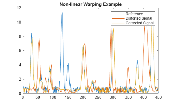
Plot the reference signal, distorted signal, and warped (corrected) signal.
figure sig_3 = interp1(time,sig_2,interp1(i,j,time,'pchip'),'pchip'); plot(time,sig_1,time,sig_2,time,sig_3) legend('Reference','Distorted Signal','Corrected Signal') title('Non-linear Warping Example')
Plot the real and the estimated warping functions.
figure plot(time,wf(time),time,interp1(j,i,time,'pchip')) legend('Distorting Function','Estimated Warping')
Note
For examples of using function handles for the Band
,
Gap
, and Distance
properties, see Visualizing and Preprocessing Hyphenated Mass Spectrometry Data Sets for Metabolite and Protein/Peptide Profiling.
References
[1] Myers, C.S. and Rabiner, L.R. (1981). A comparative study of several dynamic time-warping algorithms for connected word recognition. The Bell System Technical Journal 60:7, 1389–1409.
[2] Sakoe, H. and Chiba, S. (1978). Dynamic programming algorithm optimization for spoken word recognition. IEEE Trans. Acoustics, Speech and Signal Processing ASSP-26(1), 43–49.
Version History
Introduced in R2007b
See Also
msalign
| msheatmap
| mspalign
| msppresample
| msresample