sinr

Display or compute signal-to-interference-plus-noise (SINR) ratio

Syntax

sinr(txs)

sinr(txs,propmodel)

sinr(___,Name=Value)

pd = sinr(txs,___)

r = sinr(rxs,txs,___)

Description

sinr(txs) displays the signal-to-interference-plus-noise ratio (SINR) for transmitter sites txs in the current Site Viewer. The function generates map contours using SINR values that are computed for receiver site locations on the map. For each location, the signal source is the transmitter site in txs with the greatest signal strength. The remaining transmitter sites in txs with the same transmitter frequency act as sources of interference. If txs is scalar or there are no sources of interference, Site Viewer displays signal-to-noise ratio (SNR).

This function only supports plotting for antenna sites with a CoordinateSystem property value of "geographic".

sinr(txs,propmodel) displays the SINR map using the propagation model specified by propmodel.

sinr(___,Name=Value) sets properties using one or more name-value arguments, in addition to the input argument combinations in the previous syntaxes. For example, sinr(txs,MaxRange=8000) specifies the range of the SINR map region as 8000 m from the site location.

pd = sinr(txs,___) returns the computed SINR data in the propagation data object pd. This syntax ignores name-value arguments for the SINR map display and does not display data in Site Viewer.

r = sinr(rxs,txs,___) returns the SINR, in dB, computed at the receiver sites due to the transmitter sites.

Examples

SINR Map for Multiple Transmitters

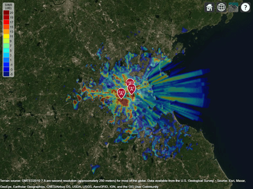
Define names and location of three sites in Boston.

name = ["Fenway Park","Faneuil Hall","Bunker Hill Monument"];
lat = [42.3467 42.3598 42.3763];
lon = [-71.0972 -71.0545 -71.0611];

Create an array of transmitter sites.

txs = txsite(Name=name, ...
    Latitude=lat, ...
    Longitude=lon, ...
    TransmitterFrequency=2.5e9);

Display the SINR map. Each location on the map is colored using the strongest signal available at that location.

sinr(txs)

Input Arguments

txs — Transmitter site

txsite object | array of txsite objects

Transmitter site, specified as a txsite object or an array of txsite objects.

This function only supports plotting antenna sites when the CoordinateSystem property is set to "geographic".

rxs — Receiver sites

rxsite object | array of rxsite objects

Receiver site, specified as a rxsite object or an array of rxsite objects.

This function only supports plotting antenna sites when the CoordinateSystem property is set to "geographic".

propmodel — Propagation model to use for path loss calculations

"freespace" | "close-in" | "rain" | "gas" | "fog" | "longley-rice" | "raytracing" | propagation model created using propagationModel | ...

Propagation model to use for the path loss calculations, specified as one of these options:

• "freespace" — Free space propagation model

• "rain" — Rain propagation model

• "gas" — Gas propagation model

• "fog" — Fog propagation model

• "close-in" — Close-in propagation model

• "longley-rice" — Longley-Rice propagation model

• "tirem" — TIREM™ propagation model

• "raytracing" — Ray tracing propagation model that uses the shooting and bouncing rays (SBR) method. When you specify a ray tracing model as input, the function incorporates multipath interference by using a phasor sum.

• A propagation model created using the propagationModel function. For example, you can create a ray tracing propagation model that uses the image method by specifying propagationModel("raytracing",Method="image").

• A composite propagation model. Create a composite propagation model from individual propagation models by using the add function. For information about the types of propagation models that can be combined, see Choose a Propagation Model.

The default depends on the coordinate system of the antenna sites and the value of the Map argument.

Coordinate System	Default Propagation Model
"geographic"	"longley-rice" when Map specifies terrain data. "freespace" when Map does not specify terrain data.
"cartesian"	"freespace" when Map specifies "none". "raytracing" when Map specifies the name of a glTF™ file, the name of an STL file, or a triangulation object. The default ray tracing model uses the shooting and bouncing rays (SBR) method.

Terrain propagation models, including "longley-rice" and "tirem", are only supported for sites with a CoordinateSystem value of "geographic".

You can also specify the propagation model by using the PropagationModel name-value argument. If you specify both propmodel and PropagationModel, the function uses the value of PropagationModel.

Name-Value Arguments

Specify optional pairs of arguments as Name1=Value1,...,NameN=ValueN, where Name is the argument name and Value is the corresponding value. Name-value arguments must appear after other arguments, but the order of the pairs does not matter.

Example: sinr(txs,MaxRange=8000) specifies the range of the SINR map region as 8000 m from the site location.

Before R2021a, use commas to separate each name and value, and enclose Name in quotes.

Example: sinr(txs,"MaxRange",8000) specifies the range of the SINR map region as 8000 m from the site location.

General

SignalSource — Signal source of interest

"strongest" (default) | txsite object | array of txsite objects

Signal source of interest, specified as one of these options:

• "strongest" — Color each location on the map using the strongest signal available at that location.

• A txsite object — Color all locations using the specified transmitter site as the signal source of interest.

• An array of txsite objects — Color each receiver site specified by rxs using the corresponding transmitter site as the signal source of interest. The sizes of the array and rxs must match.

PropagationModel — Propagation model to use for path loss calculations

"freespace" | "close-in" | "rain" | "gas" | "fog" | "longley-rice" | "raytracing" | propagation model created using propagationModel | ...

Propagation model to use for the path loss calculations, specified as one of these options:

• "freespace" — Free space propagation model

• "rain" — Rain propagation model

• "gas" — Gas propagation model

• "fog" — Fog propagation model

• "close-in" — Close-in propagation model

• "longley-rice" — Longley-Rice propagation model

• "tirem" — TIREM propagation model

• "raytracing" — Ray tracing propagation model that uses the shooting and bouncing rays (SBR) method. When you specify a ray tracing model as input, the function incorporates multipath interference by using a phasor sum.

• A propagation model created using the propagationModel function. For example, you can create a ray tracing propagation model that uses the image method by specifying propagationModel("raytracing",Method="image").

• A composite propagation model. Create a composite propagation model from individual propagation models by using the add function. For information about the types of propagation models that can be combined, see Choose a Propagation Model.

The default depends on the coordinate system of the antenna sites and the value of the Map argument.

Coordinate System	Default Propagation Model
"geographic"	"longley-rice" when Map specifies terrain data. "freespace" when Map does not specify terrain data.
"cartesian"	"freespace" when Map specifies "none". "raytracing" when Map specifies the name of a glTF file, the name of an STL file, or a triangulation object. The default ray tracing model uses the shooting and bouncing rays (SBR) method.

Terrain propagation models, including "longley-rice" and "tirem", are only supported for sites with a CoordinateSystem value of "geographic".

You can also specify the propagation model by using the propmodel argument. If you specify both propmodel and PropagationModel, the function uses the value of PropagationModel.

ReceiverNoisePower — Total noise power at receiver in dBm

-107 (default) | scalar

Total noise power at receiver, specified as a scalar in dBm. The default value assumes that the receiver bandwidth is 1 MHz and receiver noise figure is 7 dB.

The receiver noise in dBm, N, is represented by the equation:

$$N=-174+10*\log (B)+F$$

where:

• B is the receiver bandwidth in Hz.

• F is the noise figure in dB.

ReceiverGain — Receiver gain in dBi

2.1 (default) | scalar

Mobile receiver gain, specified as a scalar in dBi. The receiver gain values include the antenna gain and the system loss. If you call the function using an output argument, the default value is computed using rxs.

ReceiverAntennaHeight — Height of phase center of receiver antenna in m

1 (default) | scalar

Height above the ground of the phase center of the receiver antenna, specified as a scalar in m. If you specify an output argument, by default, the function uses the receiver sites in rxs.

Map — Map for visualization or surface data

siteviewer object | triangulation object | string scalar | character vector

Map for visualization or surface data, specified as a siteviewer object, a triangulation object, a string scalar, or a character vector. Valid and default values depend on the coordinate system.

Coordinate System	Valid Map Values	Default Map Value
"geographic"	A siteviewer object.a A terrain name, if the function is called with an output argument. Valid terrain names are: "none" — Terrain elevation is 0 everywhere. "gmted2010" — USGS GMTED2010 terrain data. This option requires an internet connection. The name of custom terrain data added using the addCustomTerrain function, specified using a string scalar or a character vector.	If the function is not called with an output, the current siteviewer object, or a new siteviewer object if none are open. By default, siteviewer objects use USGS GMTED2010 terrain data. If the function is called with an output, "gmted2010".
"cartesian"	"none" A siteviewer object. The name of a glTF file, specified using a string scalar or a character vector. The name of an STL file, specified using a string scalar or a character vector. A triangulation object.	"none"
a Alignment of boundaries and region labels are a presentation of the feature provided by the data vendors and do not imply endorsement by MathWorks®.

In most cases, if you specify this argument as a value other than a siteviewer or "none", then you must also specify an output argument.

For Plotting SINR

Values — Values of SINR for display

[-5:20] (default) | numeric vector

Values of SINR for display, specified as a numeric vector. Each value is displayed as a different colored, filled on the contour map. The function derives the contour colors using the Colormap and ColorLimits arguments.

MaxRange — Maximum range in m

numeric scalar

Maximum range of the SINR map from each transmitter site, specified as a positive numeric scalar in m representing great circle distance. MaxRange defines the region of interest on the map to plot. The default value depends on the type of propagation model.

Type of Propagation Model	Default Maximum Range
Atmospheric or empirical	30 km
Terrain	The minimum of 30 km and the distance to the furthest building
Ray tracing	500 m

For more information about the types of propagation models, see Choose a Propagation Model.

Data Types: double

Resolution — Resolution of receiver site locations used to compute SINR values

"auto" (default) | numeric scalar

Resolution of receiver site locations used to compute SINR values, specified as "auto" or a numeric scalar in m. The resolution defines the maximum distance between the locations. If the resolution is "auto", the function computes a value scaled to MaxRange. Decreasing the resolution increases the quality of the SINR map and the time required to create it.

Colormap — Colormap for filled contours

jet (default) | colormap name | M-by-3 array of RGB triplets

Colormap for the filled contours, specified as a colormap name or as an M-by-3 array of RGB triplets that define M individual colors.

This table lists the colormap names.

Colormap Name	Color Scale
parula
turbo
hsv
hot
cool
spring
summer
autumn
winter
gray
bone
copper
pink
sky (since R2023a)
abyss (since R2023b)
nebula (since R2025a)
jet
lines
colorcube
prism
flag
white

Data Types: char | string | double

ColorLimits — Color limits for colormap

[-5 20] (default) | two-element vector

Color limits for the colormap, specified as a two-element vector of the form [cmin cmax]. The value of cmin must be less than cmax.

The color limits indicate the SINR values that map to the first and last colors in the colormap.

ShowLegend — Show signal strength color legend on map

true (default) | false

Show signal strength color legend on map, specified as true or false.

Data Types: logical

Transparency — Transparency of SINR map

0.4 (default) | numeric scalar

Transparency of the SINR map, specified as a numeric scalar in the range 0 to 1. 0 is transparent and 1 is opaque.

Output Arguments

pd — SINR data

propagationData object

SINR data, returned as a propagationData object with these properties:

• Name has a value of 'SINR Data'.

• Data contains a table with Latitude, Longitude, and SINR table variables.

• DataVariableName has a value of 'SINR'.

r — SINR at the receiver

numeric vector (default)

SINR at the receiver due to the transmitter sites, returned as a numeric vector. The length of the vector matches the number of receiver sites.

Data Types: double

Limitations

When you specify a RayTracing object as input to the sinr function, the value of the MaxNumDiffractions property must be 0 or 1.

References

[1] International Telecommunications Union Radiocommunication Sector. Effects of Building Materials and Structures on Radiowave Propagation Above About 100MHz. Recommendation P.2040. ITU-R, approved August 23, 2023. https://www.itu.int/rec/R-REC-P.2040/en.

[2] International Telecommunications Union Radiocommunication Sector. Electrical Characteristics of the Surface of the Earth. Recommendation P.527. ITU-R, approved September 27, 2021. https://www.itu.int/rec/R-REC-P.527/en.

[3] Mohr, Peter J., Eite Tiesinga, David B. Newell, and Barry N. Taylor. “Codata Internationally Recommended 2022 Values of the Fundamental Physical Constants.” NIST, May 8, 2024. https://www.nist.gov/publications/codata-internationally-recommended-2022-values-fundamental-physical-constants.

[4] "IEEE Standard Definitions of Terms for Antennas." IEEE Std 145-2013 (Revision of IEEE Std 145-1993), March 2014, 1–50. https://doi.org/10.1109/IEEESTD.2014.6758443.

Extended Capabilities

GPU Arrays

Accelerate code by running on a graphics processing unit (GPU) using Parallel Computing Toolbox™. (since R2025a)

The sinr function supports ray tracing analysis on a GPU with these usage notes and limitations:

• The function runs on the GPU when you specify a RayTracing propagation model object as input and the UseGPU property of the object is "on" or "auto".

• For information about when the GPU can accelerate ray tracing analysis, see the UseGPU property of the RayTracing object.

• In some cases, the GPU and local CPU results can differ due to small differences in algorithms and hardware implementations.

For an example that shows how to perform ray tracing analysis on a GPU, see Accelerate Ray Tracing Analysis Using GPU.

Version History

Introduced in R2019b

R2026a: Ray tracing functions use improved polarization algorithm

Ray tracing functions calculate path loss and phase shift using the polarization convention described by IEEE^® Standard 145-2013 [4], such that MATLAB^® expects the polarization of the receiver antenna to be defined as if it were transmitting.

As a result of this change, when used with polarized antennas, the sinr function can return different values in R2026a compared to previous releases.

R2026a: Propagation models that combine rain and ray tracing use improved algorithm

Propagation models that combine Rain objects and RayTracing objects use an improved algorithm, where the model calculates propagation loss from rain for each ray path segment.

As a result of this change, the sinr function can return different values in R2026a compared to previous releases.

R2025a: Ray tracing functions perform analysis using additional materials

When calculating SINR using ray tracing models, the sinr function performs the ray tracing analysis using additional materials. For a list of supported materials and more information about the electromagnetic properties used by ray tracing models, see Properties of Ray Tracing Materials.

As a result of this change, depending on the materials in the scene, the sinr function can return different values in R2025a compared to previous releases.

R2025a: Ray tracing functions use improved algorithms

When calculating SINR using ray tracing models, the sinr function uses improved algorithms and constant values.

• The SBR method uses additional edges in the scene as candidates for diffraction. As a result, the SBR method can find more rays in R2025a compared to previous releases.

• When you specify transmitters and receivers that have polarized antennas from Antenna Toolbox™ or Phased Array System Toolbox™, the function calculates the phase shifts of rays using an improved algorithm that differently incorporates the far-field patterns of the antennas.

• The function uses the constant values that are recommended by the 2022 Committee on Data of the International Science Council (CODATA) adjustment of fundamental constants [3]. In previous releases, the function used constant values from International Telecommunication Union Recommendations (ITU-R) P.2040 and P.527.

As a result of these changes, the sinr function can return different values in R2025a compared to previous releases.

R2025a: Improved performance in scenes with buildings

The sinr function shows improved performance in scenes with buildings when you specify a RayTracing propagation model object as input.

For example, the following code creates a coverage map for two antenna sites in an urban scene by using the sinr function and a RayTracing propagation model object created using the propagationModel function. The code that creates the SINR map is about 1.7x faster in R2025a than in R2024b.

function t = timingTest
    % Create Site Viewer and sites
    sv = siteviewer(Buildings="chicago.osm",Terrain="none");
    tx = txsite(Latitude=[41.88 41.8807], ...
        Longitude=[-87.6295 -87.6308]);

    % Create RayTracing object
    pm = propagationModel("raytracing");

    % Create SINR map
    t0 = tic;
    sinr(tx,pm)
    t = toc(t0);

    % Close Site Viewer
    close(sv)
end

The approximate execution times are:

• R2025a: 6.8 s

• R2024b: 11.6 s

This code was timed on a Windows^® 11, AMD EPYC™ 74F3 24-Core Processor @ 3.19 GHz test system by calling the function timingTest.

You can download the OpenStreetMap file used in this example from https://www.openstreetmap.org, which provides access to crowd-sourced map data all over the world. The data is licensed under the Open Data Commons Open Database License (ODbL), https://opendatacommons.org/licenses/odbl/.

R2024a: Ray tracing functions model materials using updated ITU recommendations

When calculating SINR using ray tracing models, the sinr function models materials using the methods and equations in ITU-R P.2040-3 [1] and ITU-R P.527-5 through ITU-R P.527-6 [2].

In previous releases, the function used ITU-R P.2040-1. As a result of these changes, the sinr function can return different values in R2024a compared to previous releases.

R2023b: Perform ray tracing analysis with multiple materials in the same scene

The sinr function performs ray tracing analysis with multiple materials in the same scene when:

• You create the scene from a glTF file, and specify the propmodel input argument as "raytracing" or a RayTracing propagation model object with its SurfaceMaterial property set to "auto" (the default).

• You create the scene from an OpenStreetMap^® file or a geospatial table, and you specify the propmodel input argument as "raytracing" or a RayTracing propagation model object with its BuildingsMaterial property set to "auto" (the default).

The sinr function performs the ray tracing analysis using the materials stored in the file or table. If the file or table does not specify materials, or if the file or table specifies a material that the ray tracing analysis does not support, then the function uses concrete instead of the absent or unsupported material.

As a result, the sinr function can return different values in R2023b compared to previous releases. To avoid using the materials stored in the file or table, create a RayTracing object (by using the propagationModel function) and set its SurfaceMaterial property to "plasterboard" and its BuildingsMaterial property to "concrete". Then, use the object as input to the sinr function.

R2023b: Ray tracing analysis with SBR method shows improved performance in complex scenes

The sinr function shows improved performance with complex scenes when you specify a RayTracing propagation model object that uses the shooting and bouncing rays (SBR) method as input.

The time that MATLAB requires to perform ray tracing analysis depends on the scene and on the properties of the RayTracing object, such as the AngularSeparation, MaxNumDiffractions, MaxNumReflections, MaxAbsolutePathLoss, and MaxRelativePathLoss properties. In some cases, with moderate values of the MaxAbsolutePathLoss and MaxRelativePathLoss properties, the ray tracing analysis can be more than 2x faster in R2023b than in R2023a.

R2023a: Ray tracing models discard paths based on path loss

Ray tracing propagation models discard propagation paths based on path loss thresholds. By default, when you specify the propmodel input argument as "raytracing" or a RayTracing object, the propagation model discards paths that are more than 40 dB weaker than the strongest path.

As a result, the sinr function can return different values in R2023a compared to previous releases. To avoid discarding paths based on relative path loss thresholds, create a RayTracing object (by using the propagationModel function) and set its MaxRelativePathLoss property to Inf. Then, use the object as input to the sinr function.

R2022b: Ray tracing functions consider multipath interference

When calculating SINR using ray tracing models, the sinr function now incorporates multipath interference by using a phasor sum. In previous releases, the function used a power sum. As a result, the calculations in R2022b are more accurate than in previous releases.

R2021b: "raytracing" propagation models use SBR method

Starting in R2021b, when you use the sinr function and specify the propmodel argument or PropagationModel name-value argument as "raytracing", the function uses the shooting and bouncing rays (SBR) method and calculates up to two reflections. In previous releases, the sinr function uses the image method and calculates up to one reflection.

To display or compute the SINR using the image method instead, create a propagation model by using the propagationModel function. Then, use the sinr function with the propagation model as input. This example shows how to update your code.

pm = propagationModel("raytracing","Method","image");
sinr(txs,pm)

For information about the SBR and image methods, see Choose a Propagation Model.

Starting in R2021b, all RF Propagation functions use the SBR method by default and calculate up to two reflections. For more information, see Default modeling method is shooting and bouncing rays method.