showStateInfo

State vector map for sparse model

Syntax

showStateInfo(sys)

Description

showStateInfo(sys) prints a state vector map of the x or q vectors, that is, how they are partitioned into components, interfaces, and signals.

For sparss models, showStateInfo maps the content of the state vector x back to individual components and internal signals. Here, Component refers to the sub-components or sub-structures that were combined into sys. The Signal group includes all signals flowing between components, for example, in series or feedback connections.

For mechss models, showStateInfo maps the content of the vector q of generalized degrees of freedom in terms of components, interfaces, and signals. The Interface group includes all DAE variables arising from physical couplings between components (see addInterface and assemble).

Examples

Sparse Second-Order Model in a Feedback Loop

For this example, consider sparseSOSignal.mat that contains a sparse second-order model. Define an actuator, sensor, and controller and connect them together with the plant in a feedback loop.

Load the sparse matrices and create the mechss object.

load sparseSOSignal.mat
plant = mechss(M,C,K,B,F,[],[],'Name','Plant');

Next, create an actuator and sensor using transfer functions.

act = tf(1,[1 0.5 3],'Name','Actuator');
sen = tf(1,[0.02 7],'Name','Sensor');

Create a PID controller object for the plant.

con = pid(1,1,0.1,0.01,'Name','Controller');

Use the feedback command to connect the plant, sensor, actuator, and controller in a feedback loop.

sys = feedback(sen*plant*act*con,1)

Sparse continuous-time second-order model with 1 outputs, 1 inputs, and 7111 degrees of freedom.
Model Properties

Use "spy" and "showStateInfo" to inspect model structure. 
Type "help mechssOptions" for available solver options for this model.

The resultant system sys is a mechss object since mechss objects take precedence over all other model object types.

Use showStateInfo to view the component and signal groups.

showStateInfo(sys)

The state groups are:

    Type          Name       Size
  -------------------------------
  Component      Sensor         1
  Component      Plant       7102
  Signal                        1
  Component     Actuator        2
  Signal                        1
  Component    Controller       2
  Signal                        1
  Signal                        1

Use xsort to sort the components and signals, and then view the component and signal groups.

sysSort = xsort(sys);
showStateInfo(sysSort)

The state groups are:

    Type          Name       Size
  -------------------------------
  Component      Sensor         1
  Component      Plant       7102
  Component     Actuator        2
  Component    Controller       2
  Signal                        4

Observe that the components are now ordered before the signal partition. The signals are now sorted and grouped together in a single partition.

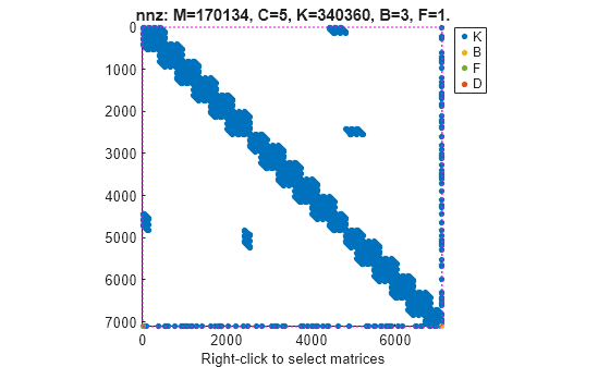
You can also visualize the sparsity pattern of the resultant system using spy.

spy(sysSort)

Physical Connections Between Components in Sparse Second-Order Model

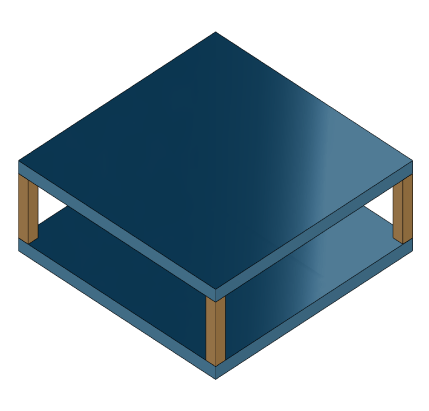
For this example, consider a structural model that consists of two square plates connected with pillars at each vertex as depicted in the figure below. The lower plate is attached rigidly to the ground while the pillars are attached rigidly to each vertex of the square plate.

Load the finite element model matrices contained in platePillarModel.mat and create the sparse second-order model representing the above system.

load('platePillarModel.mat')

Define interfaces.

Plate1 = mechss(M1,[],K1,B1,F1,'Name','Plate1');
Plate2 = mechss(M2,[],K2,B2,F2,'Name','Plate2');

Now, load the interfaced degree of freedom (DOF) index data from dofData.mat and use interface to create the physical connections between the two plates and the four pillars. dofs is a 6x7 cell array where the first two rows contain DOF index data for the first and second plates while the remaining four rows contain index data for the four pillars. By default, the function uses dual-assembly method of physical coupling.

load('dofData.mat','dofs')
for ct=1:4
    % Plates to pillars
    Plate1 = addInterface(Plate1,"Pillar"+ct,dofs{1,2+ct});
    Plate2 = addInterface(Plate2,"Pillar"+ct,dofs{2,2+ct});
end

P = cell(4,1);
for ct=1:4
    % Pillars to plates
    P{ct} = mechss(Mp,[],Kp,Bp,Fp,'Name',"Pillar"+ct);
    P{ct} = addInterface(P{ct},"TopMount",dofs{2+ct,1});
    P{ct} = addInterface(P{ct},"BottomMount",dofs{2+ct,2});
end
% Plate 2 to ground

Specify connection between the bottom plate and the ground.

Plate2 = addInterface(Plate2,"Ground",dofs{2,7});

% Assemble
model = append(Plate1,Plate2,P{:});

Use showStateInfo to confirm the physical interfaces.

showStateInfo(model)

The state groups are:

    Type        Name      Size
  ----------------------------
  Component    Plate1     2646
  Component    Plate2     2646
  Component    Pillar1     132
  Component    Pillar2     132
  Component    Pillar3     132
  Component    Pillar4     132

sysConDual = model;
for ct=1:4
    sysConDual = assemble(sysConDual,"Plate1:Pillar"+ct,"Pillar"+ct+":TopMount"');
    sysConDual = assemble(sysConDual,"Plate2:Pillar"+ct,"Pillar"+ct+":BottomMount");
end
sysConDual = assemble(sysConDual,"Plate2:Ground","Ground");

Use showStateInfo to confirm the physical interfaces.

showStateInfo(sysConDual)

The state groups are:

    Type                      Name                   Size
  -------------------------------------------------------
  Component                  Plate1                  2646
  Component                  Plate2                  2646
  Component                 Pillar1                   132
  Component                 Pillar2                   132
  Component                 Pillar3                   132
  Component                 Pillar4                   132
  Interface     Plate1:Pillar1-Pillar1:TopMount        12
  Interface    Plate2:Pillar1-Pillar1:BottomMount      12
  Interface     Plate1:Pillar2-Pillar2:TopMount        12
  Interface    Plate2:Pillar2-Pillar2:BottomMount      12
  Interface     Plate1:Pillar3-Pillar3:TopMount        12
  Interface    Plate2:Pillar3-Pillar3:BottomMount      12
  Interface     Plate1:Pillar4-Pillar4:TopMount        12
  Interface    Plate2:Pillar4-Pillar4:BottomMount      12
  Interface           Plate2:Ground-Ground              6

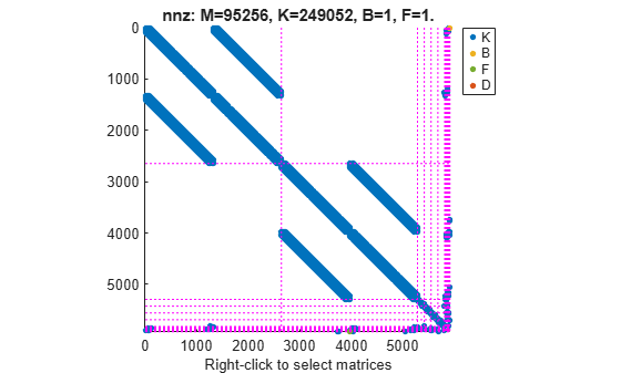
You can use spy to visualize the sparse matrices in the final model.

spy(sysConDual)

Now, specify physical connections using the primal-assembly method.

sysConPrimal = model;
for ct=1:4
    sysConPrimal = assemble(sysConPrimal,"Plate1:Pillar"+ct,"Pillar"+ct+":TopMount"',Method="primal");
    sysConPrimal = assemble(sysConPrimal,"Plate2:Pillar"+ct,"Pillar"+ct+":BottomMount",Method="primal");
end
sysConPrimal = assemble(sysConPrimal,"Plate2:Ground","Ground",Method="primal");

Use showStateInfo to confirm the physical interfaces.

showStateInfo(sysConPrimal)

The state groups are:

    Type       Name    Size
  -------------------------
  Component            5718

Primal assembly eliminates half of the redundant DOFs associated with the shared set of DOFs in the global finite element mesh.

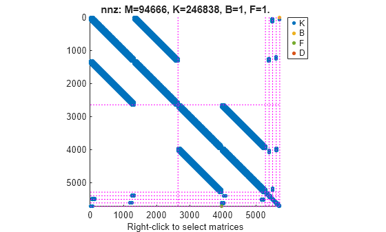
You can use spy to visualize the sparse matrices in the final model.

spy(sysConPrimal)

The data set for this example was provided by Victor Dolk from ASML.

Input Arguments

sys — Sparse state-space model

sparss model object | mechss model object

Sparse state-space model, specified as a sparss or mechss model object.

Version History

Introduced in R2020b