zpk
Zero-pole-gain model
Description
Use zpk to create zero-pole-gain models, or to convert dynamic system models to zero-pole-gain
form.
Zero-pole-gain models are a representation of transfer functions in factorized form. For example, consider the following continuous-time SISO transfer function:
G(s) can be factorized into the zero-pole-gain form as:
A more general representation of the SISO zero-pole-gain model is as follows:
Here, z and p are the vectors of real-valued or complex-valued zeros and poles, and k is the real-valued or complex-valued scalar gain. For MIMO models, each I/O channel is represented by one such transfer function hij(s).
You can create a zero-pole-gain model object either by specifying the poles, zeros and
gains directly, or by converting a model of another type (such as a state-space model
ss) to zero-pole-gain form.
You can also use zpk to create generalized state-space (genss) models or uncertain state-space (uss (Robust Control Toolbox)) models.
Creation
Syntax
Description
Create ZPK Model
sys = zpk(zeros,poles,gain)zeros and
poles specified as vectors and the scalar value of
gain. The output sys is a
zpk model object storing the model data. Set
zeros or poles to [] for
systems without zeros or poles. These two inputs need not have equal length and the
model need not be proper (that is, have an excess of poles).
sys = zpk(___,PropertyName=Value)
Convert To ZPK Model
sys = zpk(ltiSys,Name=Value)zpk representation of the sparse model
ltiSys by computing zeros and poles based on one or more
specified name-value arguments. Because this method calculates zeros for each
input-output pair, it is most suitable for models with small input-output sizes. (since R2025a)
Create Variable for Rational Expression
s = zpk('s') creates a special variable s
that you can use in a rational expression to create a continuous-time zero-pole-gain
model. Using a rational expression is sometimes easier and more intuitive than
specifying polynomial coefficients.
Input Arguments
Name-Value Arguments
Output Arguments
Properties
Object Functions
The following lists contain a representative subset of the functions you can use with
zpk models. In general, any function applicable to Dynamic System Models is
applicable to a zpk object.
Examples
For this example, consider the following continuous-time SISO zero-pole-gain model:
Specify the zeros, poles and gain, and create the SISO zero-pole-gain model.
zeros = 0;
poles = [1-1i 1+1i 2];
gain = -2;
sys = zpk(zeros,poles,gain)
sys =

          -2 s
  --------------------
  (s-2) (s^2 - 2s + 2)

Continuous-time zero/pole/gain model.
Model Properties
For this example, consider the following SISO discrete-time zero-pole-gain model with 0.1s sample time:
Specify the zeros, poles, gains and the sample time, and create the discrete-time SISO zero-pole-gain model.
zeros = [1 2 3];
poles = [6 5 4];
gain = 7;
ts = 0.1;
sys = zpk(zeros,poles,gain,ts)
sys =

  7 (z-1) (z-2) (z-3)
  -------------------
   (z-6) (z-5) (z-4)

Sample time: 0.1 seconds
Discrete-time zero/pole/gain model.
Model Properties
In this example, you create a MIMO zero-pole-gain model by concatenating SISO zero-pole-gain models. Consider the following single-input, two-output continuous-time zero-pole-gain model:
Specify the MIMO zero-pole-gain model by concatenating the SISO entries.
zeros1 = 1;
poles1 = -1;
gain = 1;
sys1 = zpk(zeros1,poles1,gain)
sys1 =

  (s-1)
  -----
  (s+1)

Continuous-time zero/pole/gain model.
Model Properties
zeros2 = -2;
poles2 = [-2+1i -2-1i];
sys2 = zpk(zeros2,poles2,gain)
sys2 =

      (s+2)
  --------------
  (s^2 + 4s + 5)

Continuous-time zero/pole/gain model.
Model Properties
sys = [sys1;sys2]
sys =

  From input to output...
       (s-1)
   1:  -----
       (s+1)

           (s+2)
   2:  --------------
       (s^2 + 4s + 5)

Continuous-time zero/pole/gain model.
Model Properties
Create a zero-pole-gain model for the discrete-time, multi-input, multi-output model:
with sample time ts = 0.2 seconds.
Specify the zeros and poles as cell arrays and the gains as an array.
zeros = {[] 0;2 []};
poles = {-0.3 -0.3;-0.3 -0.3};
gain = [1 1;-1 3];
ts = 0.2;
Create the discrete-time MIMO zero-pole-gain model.
sys = zpk(zeros,poles,gain,ts)
sys =

  From input 1 to output...
          1
   1:  -------
       (z+0.3)

       - (z-2)
   2:  -------
       (z+0.3)

  From input 2 to output...
          z
   1:  -------
       (z+0.3)

          3
   2:  -------
       (z+0.3)

Sample time: 0.2 seconds
Discrete-time zero/pole/gain model.
Model Properties
Specify the zeros, poles and gain along with the sample time and create the zero-pole-gain model, specifying the state and input names using name-value pairs.
zeros = 4;
poles = [-1+2i -1-2i];
gain = 3;
ts = 0.05;
sys = zpk(zeros,poles,gain,ts,'InputName','Force')
sys =

  From input "Force" to output:
     3 (z-4)
  --------------
  (z^2 + 2z + 5)

Sample time: 0.05 seconds
Discrete-time zero/pole/gain model.
Model Properties
The number of input names must be consistent with the number of zeros.
Naming the inputs and outputs can be useful when dealing with response plots for MIMO systems.
step(sys)
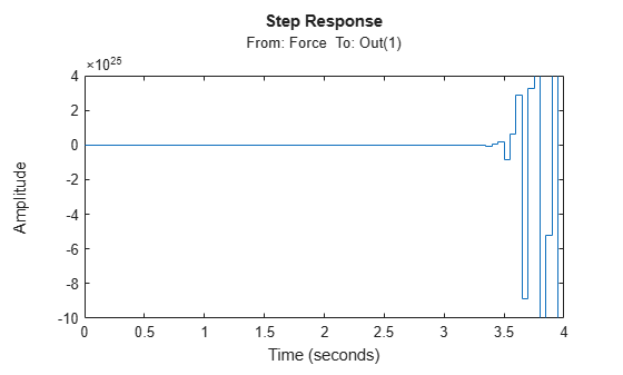
Notice the input name Force in the title of the step response plot.
For this example, create a continuous-time zero-pole-gain model using rational expressions. Using a rational expression can sometimes be easier and more intuitive than specifying poles and zeros.
Consider the following system:
To create the transfer function model, first specify s as a zpk object.
s = zpk('s')s = s Continuous-time zero/pole/gain model. Model Properties
Create the zero-pole-gain model using s in the rational expression.
sys = s/(s^2 + 2*s + 10)
sys =

         s
  ---------------
  (s^2 + 2s + 10)

Continuous-time zero/pole/gain model.
Model Properties
For this example, create a discrete-time zero-pole-gain model using a rational expression. Using a rational expression can sometimes be easier and more intuitive than specifying poles and zeros.
Consider the following system:
To create the zero-pole-gain model, first specify z as a zpk object and the sample time ts.
ts = 0.1;
z = zpk('z',ts)
z = z Sample time: 0.1 seconds Discrete-time zero/pole/gain model. Model Properties
Create the zero-pole-gain model using z in the rational expression.
sys = (z - 1) / (z^2 - 1.85*z + 0.9)
sys =

         (z-1)
  -------------------
  (z^2 - 1.85z + 0.9)

Sample time: 0.1 seconds
Discrete-time zero/pole/gain model.
Model Properties
For this example, create a zero-pole-gain model with properties inherited from another zero-pole-gain model. Consider the following two zero-pole-gain models:
For this example, create sys1 with the TimeUnit and InputDelay property set to 'minutes'.
zero1 = 0;
pole1 = [0;-8];
gain1 = 2;
sys1 = zpk(zero1,pole1,gain1,'TimeUnit','minutes','InputUnit','minutes')
sys1 =

    2 s
  -------
  s (s+8)

Continuous-time zero/pole/gain model.
Model Properties
propValues1 = [sys1.TimeUnit,sys1.InputUnit]
propValues1 = 1×2 cell
    {'minutes'}    {'minutes'}
Create the second zero-pole-gain model with properties inherited from sys1.
zero = 1;
pole = [-3,5];
gain2 = 0.8;
sys2 = zpk(zero,pole,gain2,sys1)
sys2 =

   0.8 (s-1)
  -----------
  (s+3) (s-5)

Continuous-time zero/pole/gain model.
Model Properties
propValues2 = [sys2.TimeUnit,sys2.InputUnit]
propValues2 = 1×2 cell
    {'minutes'}    {'minutes'}
Observe that the zero-pole-gain model sys2 has that same properties as sys1.
Consider the following two-input, two-output static gain matrix m:
Specify the gain matrix and create the static gain zero-pole-gain model.
m = [2,4;...
    3,5];
sys1 = zpk(m)
sys1 = From input 1 to output... 1: 2 2: 3 From input 2 to output... 1: 4 2: 5 Static gain. Model Properties
You can use static gain zero-pole-gain model sys1 obtained above to cascade it with another zero-pole-gain model.
sys2 = zpk(0,[-1 7],1)
sys2 =

       s
  -----------
  (s+1) (s-7)

Continuous-time zero/pole/gain model.
Model Properties
sys = series(sys1,sys2)
sys =

  From input 1 to output...
           2 s
   1:  -----------
       (s+1) (s-7)

           3 s
   2:  -----------
       (s+1) (s-7)

  From input 2 to output...
           4 s
   1:  -----------
       (s+1) (s-7)

           5 s
   2:  -----------
       (s+1) (s-7)

Continuous-time zero/pole/gain model.
Model Properties
For this example, compute the zero-pole-gain model of the following state-space model:
Create the state-space model using the state-space matrices.
A = [-2 -1;1 -2];
B = [1 1;2 -1];
C = [1 0];
D = [0 1];
ltiSys = ss(A,B,C,D);
Convert the state-space model ltiSys to a zero-pole-gain model.
sys = zpk(ltiSys)
sys =

  From input 1 to output:
        s
  --------------
  (s^2 + 4s + 5)

  From input 2 to output:
  (s^2 + 5s + 8)
  --------------
  (s^2 + 4s + 5)

Continuous-time zero/pole/gain model.
Model Properties
You can use a for loop to specify an array of zero-pole-gain models.
First, pre-allocate the zero-pole-gain model array with zeros.
sys = zpk(zeros(1,1,3));
The first two indices represent the number of outputs and inputs for the models, while the third index is the number of models in the array.
Create the zero-pole-gain model array using a rational expression in the for loop.
s = zpk('s');
for k = 1:3
    sys(:,:,k) = k/(s^2+s+k);
end
sys
sys(:,:,1,1) =

        1
  -------------
  (s^2 + s + 1)


sys(:,:,2,1) =

        2
  -------------
  (s^2 + s + 2)


sys(:,:,3,1) =

        3
  -------------
  (s^2 + s + 3)

3x1 array of continuous-time zero/pole/gain models.
Model Properties
For this example, extract the measured and noise components of an identified polynomial model into two separate zero-pole-gain models.
Load the Box-Jenkins polynomial model ltiSys in identifiedModel.mat.
load('identifiedModel.mat','ltiSys');
ltiSys is an identified discrete-time model of the form: , where represents the measured component and the noise component.
Extract the measured and noise components as zero-pole-gain models.
sysMeas = zpk(ltiSys,'measured') sysMeas =
From input "u1" to output "y1":
-0.14256 z^-1 (1-1.374z^-1)
z^(-2) * -----------------------------
(1-0.8789z^-1) (1-0.6958z^-1)
Sample time: 0.04 seconds
Discrete-time zero/pole/gain model.
Model Properties
sysNoise = zpk(ltiSys,'noise')sysNoise =
From input "v@y1" to output "y1":
0.045563 (1+0.7245z^-1)
--------------------------------------------
(1-0.9658z^-1) (1 - 0.0602z^-1 + 0.2018z^-2)
Input groups:
Name Channels
Noise 1
Sample time: 0.04 seconds
Discrete-time zero/pole/gain model.
Model Properties
The measured component can serve as a plant model, while the noise component can be used as a disturbance model for control system design.
For this example, create a SISO zero-pole-gain model with an input delay of 0.5 seconds and an output delay of 2.5 seconds.
zeros = 5;
poles = [7+1i 7-1i -3];
gains = 1;
sys = zpk(zeros,poles,gains,'InputDelay',0.5,'OutputDelay',2.5)
sys =

                      (s-5)
  exp(-3*s) * ----------------------
              (s+3) (s^2 - 14s + 50)

Continuous-time zero/pole/gain model.
Model Properties
You can also use the get command to display all the properties of a MATLAB object.
get(sys)
                Z: {[5]}
                P: {[3×1 double]}
                K: 1
    DisplayFormat: 'roots'
         Variable: 's'
          IODelay: 0
       InputDelay: 0.5000
      OutputDelay: 2.5000
        InputName: {''}
        InputUnit: {''}
       InputGroup: [1×1 struct]
       OutputName: {''}
       OutputUnit: {''}
      OutputGroup: [1×1 struct]
            Notes: [0×1 string]
         UserData: []
             Name: ''
               Ts: 0
         TimeUnit: 'seconds'
     SamplingGrid: [1×1 struct]
For more information on specifying time delay for an LTI model, see Specifying Time Delays.
For this example, design a 2-DOF PID controller with a target bandwidth of 0.75 rad/s for a system represented by the following zero-pole-gain model:
Create a zero-pole-gain model object sys using the zpk command.
zeros = [];
poles = [-0.25+0.2i;-0.25-0.2i];
gain = 1;
sys = zpk(zeros,poles,gain)
sys =

            1
  ---------------------
  (s^2 + 0.5s + 0.1025)

Continuous-time zero/pole/gain model.
Model Properties
Using the target bandwidth, use pidtune to generate a 2-DOF controller.
wc = 0.75;
C2 = pidtune(sys,'PID2',wc)
C2 =
1
u = Kp (b*r-y) + Ki --- (r-y) + Kd*s (c*r-y)
s
with Kp = 0.512, Ki = 0.0975, Kd = 0.574, b = 0.38, c = 0
Continuous-time 2-DOF PID controller in parallel form.
Model Properties
Using the type 'PID2' causes pidtune to generate a 2-DOF controller, represented as a pid2 object. The display confirms this result. The display also shows that pidtune tunes all controller coefficients, including the setpoint weights b and c, to balance performance and robustness.
For interactive PID tuning in the Live Editor, see the Tune PID Controller Live Editor task. This task lets you interactively design a PID controller and automatically generates MATLAB code for your live script.
For interactive PID tuning in a standalone app, use PID Tuner. See PID Controller Design for Fast Reference Tracking for an example of designing a controller using the app.
Since R2025a
This example shows how to obtain a truncated zero-pole-gain model of a sparse state-space model. This example uses a sparse model obtained from linearizing a thermal model of heat distribution in a circular cylindrical rod.
Load the model data.
load cylindricalRod.mat
sys = sparss(A,B,C,D,E);
w = logspace(-7,-1,20);
size(sys)
Sparse state-space model with 3 outputs, 1 inputs, and 7522 states.
Analyze the frequency response of the model.
sigmaplot(sys,w)
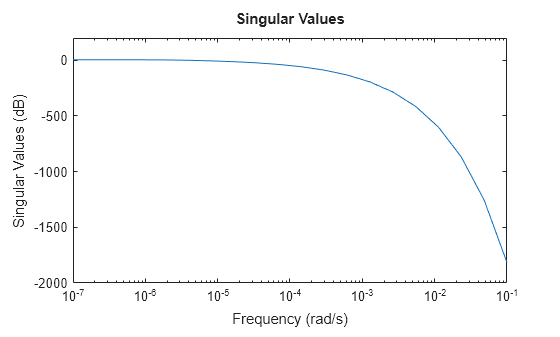
To obtain a truncated approximation, use zpk and specify the frequency band of focus. For this model, you can use a frequency range from 0 rad/s to 0.01 rad/s to obtain the low-order approximation.
zsys = zpk(sys,Focus=[0 1e-2],Display="off");Compare the frequency response.
sigmaplot(sys,zsys,w)

This thermal model has a very steep roll-off beyond 0.001 rad/s. By default, the reduced model obtained using zpk does not provide a good match for this roll-off. To mitigate this, you can use the RollOff argument of zpk and specify a minimum roll-off value beyond the frequency band of focus. Specify a roll-off slope value of -45, which corresponds to a rate of at least –900 db/decade.
zsys2 = zpk(sys,Focus=[0 1e-2],RollOff=-45,Display="off");
sigmaplot(sys,zsys2,w)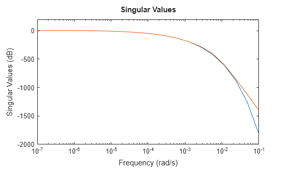
The reduced model now provides a much better approximation of the roll-off value. However, in this example, readjusting roll-off slope using zpk requires recomputing zeros and poles. This may be computationally expensive in case of large-scale models. As an alternative, you can use the zero-pole truncation method of reducespec and adjust roll-off at no extra computation cost, after the software has computed poles and zeros. For an example, see Zero-Pole Truncation of Thermal Model.
Algorithms
zpk uses the MATLAB function roots to convert transfer functions and the
functions zero and pole to convert state-space models.
To convert sparse models, zpk uses the Krylov--Schur algorithm [1] for
inverse power iterations to compute poles and zeros in the specified frequency band.
References
[1] Stewart, G. W. “A Krylov--Schur Algorithm for Large Eigenproblems.” SIAM Journal on Matrix Analysis and Applications 23, no. 3 (January 2002): 601–14. https://doi.org/10.1137/S0895479800371529.