LTV and LPV Modeling
Types of LTV and LPV Models
There are two main categories of linear time-varying (LTV) and linear parameter-varying (LPV) models:
Models specified by their data function (a MATLAB® function), also called analytic models. These are often physical models whose state-space equations are mostly linear except for a few time-varying or parameter-dependent terms. Examples of such models include the models in LPV Model of Bouncing Ball, LPV Model of Engine Throttle, Analysis of Gain-Scheduled PI Controller, and Control Design for Spinning Disks. They can also come from hand linearization of nonlinear models, as demonstrated in LPV Model of Magnetic Levitation System and Hidden Couplings in Gain-Scheduled Control.
Models interpolating linearization results either along a trajectory or over a grid of operating conditions, also called data-driven models. Each linearization captures the local linear dynamics at a given time or around a given operating point, and the interpolation provides smooth transition between these operating regimes. Examples of such models are given in Design and Validate Gain-Scheduled Controller for Nonlinear Aircraft Pitch Dynamics, LPV Approximation of Boost Converter Model, LPV Model of Magnetic Levitation Model from Batch Linearization Results, LTV Model of Two-Link Robot, and Control Design for Wind Turbine.
Technically, gridded models are a particular type of analytic models where the data function is data driven rather than formula driven. Conceptually, however, the two types of model have different origins and correspond to different modeling workflows and approximation strategies.
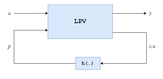
Quasi-LPV models are LPV models where the scheduling map or parameter trajectory p(t) is endogenous rather than exogenous, that is, depends on the state x and input u of the model. This creates a feedback loop between the LPV model and the scheduling map.
The lpvss
object cannot represent an entire quasi-LPV model with its scheduling map. However,
you can simulate the response of quasi-LPV models by specifying the scheduling
function as the parameter trajectory. Quasi-LPV models can represent
virtually any nonlinear system but do not turn nonlinear systems into linear ones.
Moving nonlinearities into the scheduling map can create instabilities and hide
difficulties when not done carefully (see Hidden Couplings in Gain-Scheduled Control). These
difficulties generally do not arise, however, when
p(t) changes slowly compared to the
dominant system dynamics (see the Gain-Scheduled LQG Controller example for an
illustration). Examples involving quasi-LPV simulations include: LPV Model of Magnetic Levitation System, LPV Model of Bouncing Ball, LPV Model of Engine Throttle, Design and Validate Gain-Scheduled Controller for Nonlinear Aircraft Pitch Dynamics, and Control Design for Wind Turbine.
Limitations of LPV Models
LPV approximations are most useful for systems whose behavior is nearly linear on a short time scale but nonlinear or time-varying on a longer time horizon. They tend to be less useful for systems with fast, highly nonlinear dynamics. Quasi-LPV models are most useful when the dynamics of the scheduling feedback loop are slow or benign, and least useful when these dynamics dominate those of the LPV model itself (or of any gain-scheduled control loop based on the LPV model alone).
Gridded LPV models based on linearized dynamics cannot represent hard nonlinearities such as saturations and dead zones (see Hidden Couplings in Gain-Scheduled Control for an example). They can nevertheless be coupled with static nonlinearities to recover such behaviors.
Offsets and Initial Conditions
Offsets are an important part of LTV and LPV models. The linearization of the nonlinear model
around an operating point (x0,u0) is
where
For the linearization to be a good approximation of the nonlinear maps, it must
include the offsets δ0,
x0,
u0, and
y0. The linearize (Simulink Control Design) command returns both
A, B, C,
D and the offsets when using the
StoreOffset option. This is the basis for constructing most
gridded LTV and LPV models. The ltvss and lpvss
objects automatically manage and propagate offset through interconnection operations
(feedback, connect, seriesparallel, lft) and transformations such as
c2d, d2c, and d2d.
Offsets and initial conditions matter for time response simulation. To obtain correct results and good approximations of the nonlinear behavior, it is important to:
Consider whether the input signal or step change is absolute or relative to the offset u0.
Correctly initialize the state vector. When the operating conditions (x0,u0) are equilibrium conditions, initializing the state vector to x0 and applying a step change relative to u0 ensures the simulation starts from the steady state (x0,u0) and approximates the nonlinear behavior around this condition. Use
RespConfigto specify these values in step. See Design and Validate Gain-Scheduled Controller for Nonlinear Aircraft Pitch Dynamics, LPV Model of Bouncing Ball, LPV Approximation of Boost Converter Model, LTV Model of Two-Link Robot, and LPV Model of Engine Throttle for examples.Specify the parameter trajectory, either explicitly for exogenous parameters (see LPV Approximation of Boost Converter Model, Control Design for Spinning Disks, Analysis of Gain-Scheduled PI Controller, and Gain-Scheduled LQG Controller), or implicitly as a function of t, x, u for quasi-LPV simulations (see LPV Model of Bouncing Ball, LPV Model of Engine Throttle, Design and Validate Gain-Scheduled Controller for Nonlinear Aircraft Pitch Dynamics, and Control Design for Wind Turbine). For a critical comparison of these two approaches, see LPV Model of Magnetic Levitation System and Hidden Couplings in Gain-Scheduled Control.
Incremental Form of LTV and LPV Models
When linearizing along a trajectory (x0(t),u0(t),y0(t)) satisfying the nonlinear equations
the linearized model can be expressed as
where
are the deviations from the reference trajectory. See the LTV Model of Two-Link Robot example for an illustration.
This incremental or delta form looks
simpler than the linearized form used for ltvss and
lpvss. However, it is not a valid representation of LPV models
in general. Consider, for example, an LPV model constructed from a family of
steady-state operating conditions
(x0(p),u0(p),y0(p))
satisfying for all p:
For fixed p, you can write the linearized dynamics around (x0(p),u0(p),y0(p)) as
with
This is no longer correct when p varies with time, that is, for an LPV trajectory that takes the system from one steady-state condition to another. In this case, you have:
The incremental form now has an extra term involving the time derivative of x0(p(t)), a quantity that is not readily available. This is why the linearized form is preferred.
State Consistency and State Transformation
When constructing LPV models from arrays of state-space models, ensure that the models are expressed in consistent state coordinates. For example, reordering the states for some models but not others creates state inconsistencies that invalidate the interpolated LPV model. In general, fixed state transformations preserve state consistency, while independent state transformations such as modal decompositions of individual models do not.
This does not mean that time-varying or parameter-varying transformations are disallowed. Given the LTV model
the time-varying state transformation x = T(t)z produces the equivalent model
However, the extra term explains why independent state transformations are problematic. If T(t) changes abruptly between time samples tk, the transformed model has an additional term that can be large and is not accounted for when transforming each model individually using Tk = T(tk):
In general, a varying state transformation is fine only when it varies slowly with time or parameters and the term can be neglected.
Gridded Models and Choice of Sampling Grid
A common way of representing LPV models is as an interpolated array of linear state-space models. For example, the aerodynamic behavior of an aircraft (see Design and Validate Gain-Scheduled Controller for Nonlinear Aircraft Pitch Dynamics) is often scheduled over a grid of incidence angle (α) and wind speed (V) values. For each scheduling parameter, a range of values is chosen, such as α = -20:5:20 degrees, V = 700:100:1400 m/s. For each combination of (α,V) values, a linear approximation of the aircraft behavior is obtained. The local models are connected as shown in this figure.
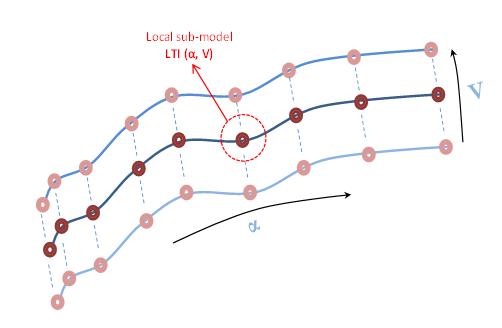
Each point represents a local LTI model, and the connecting curves represent the interpolation rules. The abscissa and ordinate of the surface are the scheduling parameters (α,V).
When using gridded LTV or LPV models to approximate nonlinear dynamics, you must determine what grid density to use and how to best distribute the grid points. The denser the grid, the more accurate the approximation, but also the more memory needed to store the matrices and offsets at all grid points. To reduce memory usage, you can prune the grid while keeping an eye on the accuracy of the LPV approximation for representative use cases (simulations for specific parameter trajectories).
You can start with a dense grid for which the LPV approximation has the desired
accuracy. Using sample, you can then sample the LPV dynamics and look for parameter
ranges where the local LTI dynamics do not change much. Using ssInterpolant, you can also try various grid densities and observe
how the LPV model fidelity deteriorates. Finally, structural information can guide
this process. For example, if the matrices and offsets depend linearly on some
parameters, the two extreme values of this parameter are enough to capture parameter
variations over an entire interval (assuming linear interpolation). By contrast, the
more nonlinear the parameter dependence is, the more grid points are needed.
For gain-scheduled control design, it is customary to use a coarser grid for the controller than for the LPV plant model. Mismatched grids are seamlessly handled by the software. See Design and Validate Gain-Scheduled Controller for Nonlinear Aircraft Pitch Dynamics, LPV Model of Magnetic Levitation Model from Batch Linearization Results, and Control Design for Wind Turbine for examples of this practice.
Optimizing LPV Models for Fast Simulation and Code Generation
LPV models can provide low-complexity approximations of high-fidelity models that
support fast simulation and code generation. When the original model is a
high-fidelity nonlinear model, batch linearization over a dense grid of operating
conditions provides the raw material for building a gridded LPV approximation. When
the original model is an analytic LPV model, it can be turned into a gridded LPV
model using ssInterpolant. Using
ssInterpolant, you can then resample the gridded LPV model
to reduce memory usage as indicated above. Finally, the gridded LPV model can be
discretized with c2d, since discrete-time models tend to
simulate faster and be more amenable to code generation and deployment. See LTV Model of Two-Link Robot and LPV Approximation of Boost Converter Model for
examples.
Other Considerations
LTV and LPV models do not commute even in the SISO case. In a gain-scheduled PI controller, for example, placing the gain-scheduled integral gain before or after the integrator is not the same, as illustrated in the Analysis of Gain-Scheduled PI Controller example.
See Also
lpvss | ltvss | sample | ssInterpolant | LPV System