Time Series Forecasting Using Deep Learning

This example shows how to forecast time series data using a long short-term memory (LSTM) network.

An LSTM network is a recurrent neural network (RNN) that processes input data by looping over time steps and updating the RNN state. The RNN state contains information remembered over all previous time steps. You can use an LSTM neural network to forecast subsequent values of a time series or sequence using previous time steps as input. To train an LSTM neural network for time series forecasting, train a regression LSTM neural network with sequence output, where the responses (targets) are the training sequences with values shifted by one time step. In other words, at each time step of the input sequence, the LSTM neural network learns to predict the value of the next time step.

There are two methods of forecasting: open loop and closed loop forecasting.

• Open loop forecasting — Predict the next time step in a sequence using only the input data. When making predictions for subsequent time steps, you collect the true values from your data source and use those as input. For example, say you want to predict the value for time step $$t$$ of a sequence using data collected in time steps 1 through $$t-1$$. To make predictions for time step $$t+1$$, wait until you record the true value for time step $$t$$ and use that as input to make the next prediction. Use open loop forecasting when you have true values to provide to the RNN before making the next prediction.

• Closed loop forecasting — Predict subsequent time steps in a sequence by using the previous predictions as input. In this case, the model does not require the true values to make the prediction. For example, say you want to predict the values for time steps $$t$$ through $$t+k$$ of the sequence using data collected in time steps 1 through $$t-1$$ only. To make predictions for time step $$i$$, use the predicted value for time step $$i-1$$ as input. Use closed loop forecasting to forecast multiple subsequent time steps or when you do not have the true values to provide to the RNN before making the next prediction.

This figure shows an example sequence with forecasted values using closed loop prediction.

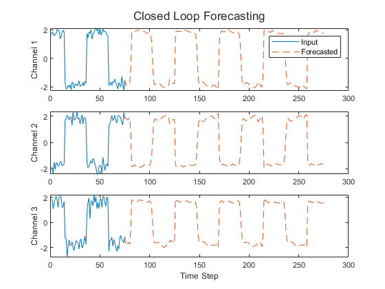
This example uses the Waveform data set, which contains 1000 synthetically generated waveforms of varying lengths with three channels. The example trains an LSTM neural network to forecast future values of the waveforms given the values from previous time steps using both closed loop and open loop forecasting.

Tip: To interactively build, train, and compare models for time series forecasting, use the Time Series Modeler app.

Load Data

Load the example data from WaveformData.mat. The data is a numObservations-by-1 cell array of sequences, where numObservations is the number of sequences. Each sequence is a numTimeSteps-by-numChannels numeric array, where numTimeSteps is the number of time steps of the sequence and numChannels is the number of channels of the sequence.

load WaveformData

View the sizes of the first few sequences.

data(1:4)

ans=4×1 cell array
    {103×3 double}
    {136×3 double}
    {140×3 double}
    {124×3 double}

View the number of channels. To train the LSTM neural network, each sequence must have the same number of channels.

numChannels = size(data{1},2)

numChannels = 
3

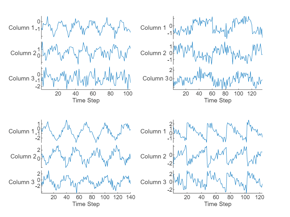
Visualize the first few sequences in a plot.

figure
tiledlayout(2,2)
for i = 1:4
    nexttile
    stackedplot(data{i})

    xlabel("Time Step")
end

Split the data into training and test partitions using the trainingPartitions function, which is attached to this example as a supporting file. To access this function, open the example as a live script. Use 90% of the data for training and the remaining 10% for testing.

numObservations = numel(data);
[idxTrain,idxTest] = trainingPartitions(numObservations,[0.9 0.1]);
dataTrain = data(idxTrain);
dataTest = data(idxTest);

Prepare Data for Training

To forecast the values of future time steps of a sequence, specify the targets as the training sequences with values shifted by one time step. Do not include the final time step in the training sequences. In other words, at each time step of the input sequence, the LSTM neural network learns to predict the value of the next time step. The predictors are the training sequences without the final time step.

numObservationsTrain = numel(dataTrain);
XTrain = cell(numObservationsTrain,1);
TTrain = cell(numObservationsTrain,1);

for n = 1:numObservationsTrain
    X = dataTrain{n};
    XTrain{n} = X(1:end-1,:);
    TTrain{n} = X(2:end,:);
end

Define LSTM Neural Network Architecture

Create an LSTM regression neural network.

• Use a sequence input layer with an input size that matches the number of channels of the input data. Normalize the input data using $$Z$$-score normalization.

• Use an LSTM layer with 128 hidden units. The number of hidden units determines how much information is learned by the layer. Using more hidden units can yield more accurate results but can be more likely to lead to overfitting to the training data.

• To output sequences with the same number of channels as the input data, include a fully connected layer with an output size that matches the number of channels of the input data.

• In this example, the training process automatically normalizes the training targets using the NormalizeTargets training option (introduced in R2026a). Using normalized targets helps stabilize training and results in training predictions that closely match the normalized targets. To make the neural network output predictions in the space of unnormalized values at prediction time, include an inverse normalization layer (introduced in R2026a). Before R2026a: To stabilize training, normalize the predictors and targets manually before you train the neural network.

layers = [
    sequenceInputLayer(numChannels,Normalization="zscore")
    lstmLayer(128)
    fullyConnectedLayer(numChannels)
    inverseNormalizationLayer];

Specify Training Options

Specify the training options. Choosing among the options requires empirical analysis. To explore different training option configurations by running experiments, you can use the Experiment Manager app.

• Train using Adam optimization.

• Automatically normalize the training targets using the NormalizeTargets option (introduced in R2026a). Before R2026a: To stabilize training, normalize the predictors and targets manually before you train the neural network.

• Train for 200 epochs. For larger data sets, you might not need to train for as many epochs for a good fit.

• In each mini-batch, left-pad the sequences so they have the same length. Left-padding prevents the RNN from predicting padding values at the ends of sequences.

• Shuffle the data every epoch.

• Display the training progress in a plot.

• Disable the verbose output.

options = trainingOptions("adam", ...
    NormalizeTargets=true, ...
    MaxEpochs=200, ...
    SequencePaddingDirection="left", ...
    Shuffle="every-epoch", ...
    Plots="training-progress", ...
    Verbose=false);

Train Recurrent Neural Network

Train the LSTM neural network using the trainnet function. For regression, use mean squared error (MSE) loss. By default, the trainnet function uses a GPU if one is available. Using a GPU requires a Parallel Computing Toolbox™ license and a supported GPU device. For information on supported devices, see GPU Computing Requirements (Parallel Computing Toolbox). Otherwise, the function uses the CPU. To select the execution environment manually, use the ExecutionEnvironment training option.

net = trainnet(XTrain,TTrain,layers,"mse",options);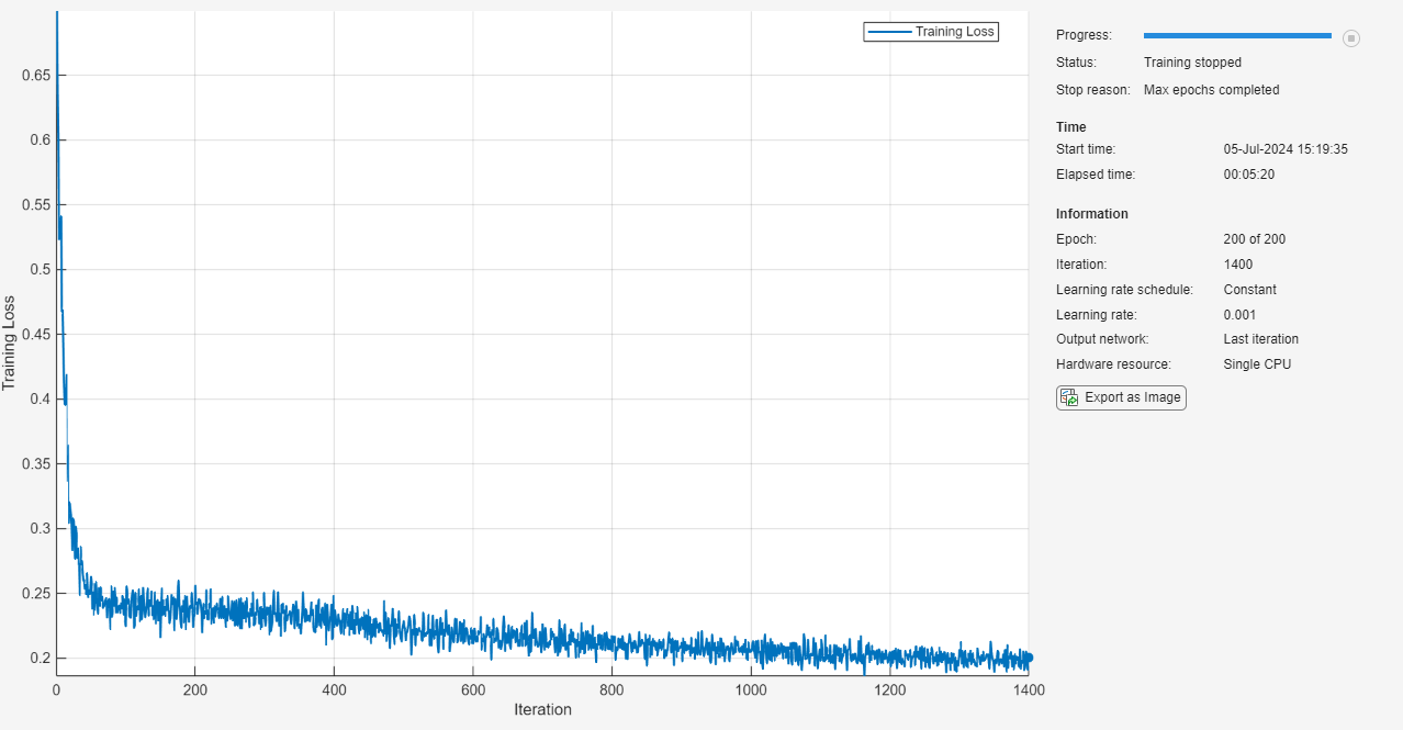

Test Recurrent Neural Network

Prepare the test data for prediction using the same steps as for the training data.

Normalize the test data using the statistics calculated from the training data. Specify the targets as the test sequences with values shifted by one time step and the predictors as the test sequences without the final time step.

numObservationsTest = numel(dataTest);
XTest = cell(numObservationsTest,1);
TTest = cell(numObservationsTest,1);

for n = 1:numObservationsTest
    X = dataTest{n};
    XTest{n} = X(1:end-1,:);
    TTest{n} = X(2:end,:);
end

Make predictions using the minibatchpredict function. By default, the minibatchpredict function uses a GPU if one is available. Pad the sequences using the same padding options as for training. For sequence-to-sequence tasks with sequences of varying lengths, return the predictions as a cell array by setting the UniformOutput option to false.

YTest = minibatchpredict(net,XTest, ...
    SequencePaddingDirection="left", ...
    UniformOutput=false);

For each test sequence, calculate the root mean squared error (RMSE) between the predictions and targets. Ignore any padding values in the predicted sequences using the lengths of the target sequences for reference.

for n = 1:numObservationsTest
    T = TTest{n};

    sequenceLength = size(T,1);    

    Y = YTest{n}(end-sequenceLength+1:end,:);

    err(n) = rmse(Y,T,"all");
end

Visualize the errors in a histogram. Lower values indicate greater accuracy.

figure
histogram(err)
xlabel("RMSE")
ylabel("Frequency")

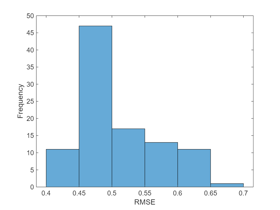
Calculate the mean RMSE over all test observations.

mean(err,"all")

ans = single

0.6618

Forecast Future Time Steps

Given an input time series or sequence, to forecast the values of multiple future time steps, use the predict function to predict time steps one at a time and update the RNN state at each prediction. For each prediction, use the previous prediction as the input to the function.

Visualize one of the test sequences in a plot.

idx = 1;
X = XTest{idx};
T = TTest{idx};

figure
stackedplot(X,DisplayLabels="Channel " + (1:numChannels))
xlabel("Time Step")
title("Test Observation " + idx)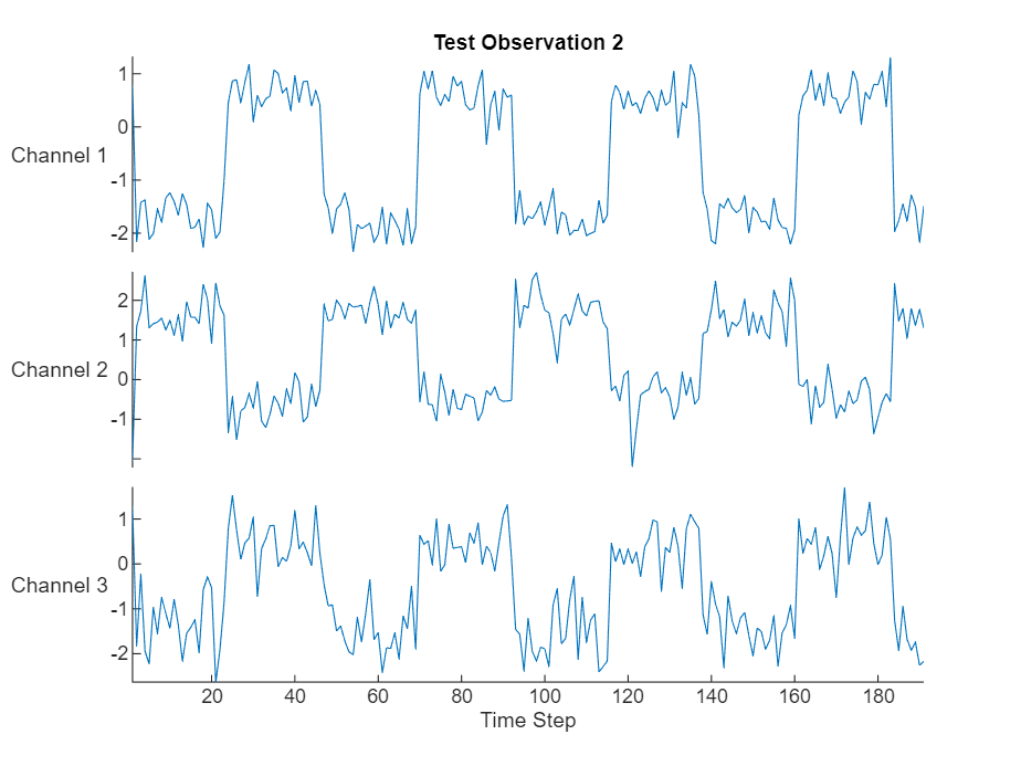

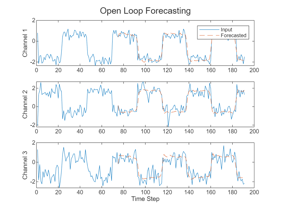
Open Loop Forecasting

Open loop forecasting predicts the next time step in a sequence using only the input data. When making predictions for subsequent time steps, you collect the true values from your data source and use those as input. For example, say you want to predict the value for time step $$t$$ of a sequence using data collected in time steps 1 through $$t-1$$. To make predictions for time step $$t+1$$, wait until you record the true value for time step $$t$$ and use that as input to make the next prediction. Use open loop forecasting when you have true values to provide to the RNN before making the next prediction.

Initialize the RNN state by first resetting the state using the resetState function, then make an initial prediction using the first few time steps of the input data. Update the RNN state using the first 75 time steps of the input data.

net = resetState(net);
offset = 75;
[Z,state] = predict(net,X(1:offset,:));
net.State = state;

To forecast further predictions, loop over time steps and make predictions using the predict function. After each prediction, update the RNN state. Forecast values for the remaining time steps of the test observation by looping over the time steps of the input data and using them as input to the RNN. The last time step of the initial prediction is the first forecasted time step.

numTimeSteps = size(X,1);
numPredictionTimeSteps = numTimeSteps - offset;
Y = zeros(numPredictionTimeSteps,numChannels);
Y(1,:) = Z(end,:);

for t = 1:numPredictionTimeSteps-1
    Xt = X(offset+t,:);
    [Y(t+1,:),state] = predict(net,Xt);
    net.State = state;
end

Compare the predictions with the input values.

figure
t = tiledlayout(numChannels,1);
title(t,"Open Loop Forecasting")

for i = 1:numChannels
    nexttile
    plot(X(:,i))
    hold on
    plot(offset:numTimeSteps,[X(offset,i) Y(:,i)'],"--")
    ylabel("Channel " + i)
end

xlabel("Time Step")
nexttile(1)
legend(["Input" "Forecasted"],Location="bestoutside")

Closed Loop Forecasting

Closed loop forecasting predicts subsequent time steps in a sequence by using the previous predictions as input. In this case, the model does not require the true values to make the prediction. For example, say you want to predict the value for time steps $$t$$ through $$t+k$$ of the sequence using data collected in time steps 1 through $$t-1$$ only. To make predictions for time step $$i$$, use the predicted value for time step $$i-1$$ as input. Use closed loop forecasting to forecast multiple subsequent time steps or when you do not have true values to provide to the RNN before making the next prediction.

Initialize the RNN state by first resetting the state using the resetState function, then make an initial prediction Z using the first few time steps of the input data. Update the RNN state using all time steps of the input data.

net = resetState(net);
offset = size(X,1);
[Z,state] = predict(net,X(1:offset,:));
net.State = state;

To forecast further predictions, loop over time steps and make predictions using the predict function. After each prediction, update the RNN state. Forecast the next 200 time steps by iteratively passing the previous predicted value to the RNN. Because the RNN does not require the input data to make any further predictions, you can specify any number of time steps to forecast. The last time step of the initial prediction is the first forecasted time step.

numPredictionTimeSteps = 200;
Y = zeros(numPredictionTimeSteps,numChannels);
Y(1,:) = Z(end,:);

for t = 2:numPredictionTimeSteps
    [Y(t,:),state] = predict(net,Y(t-1,:));
    net.State = state;
end

Visualize the forecasted values in a plot.

numTimeSteps = offset + numPredictionTimeSteps;

figure
t = tiledlayout(numChannels,1);
title(t,"Closed Loop Forecasting")

for i = 1:numChannels
    nexttile
    plot(X(1:offset,i))
    hold on
    plot(offset:numTimeSteps,[X(offset,i) Y(:,i)'],"--")
    ylabel("Channel " + i)
end

xlabel("Time Step")
nexttile(1)
legend(["Input" "Forecasted"],Location="bestoutside")

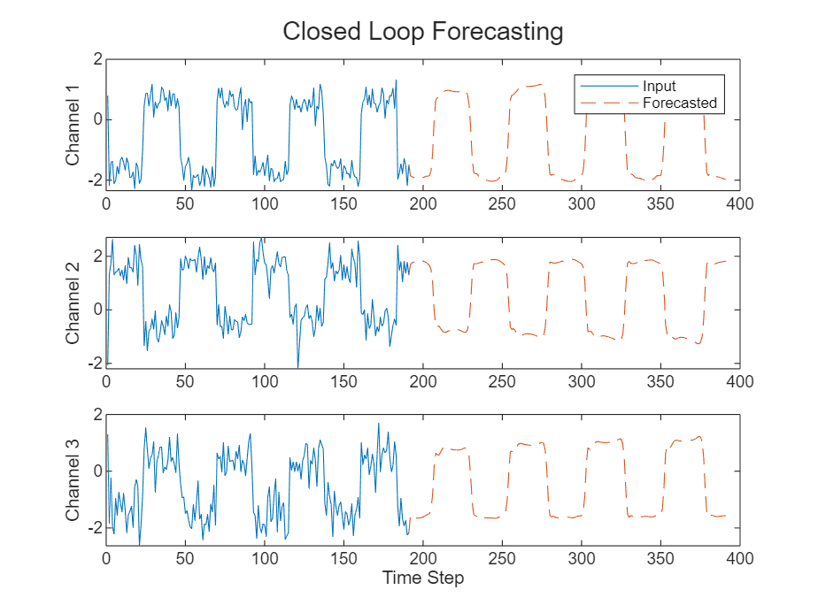
Closed loop forecasting allows you to forecast an arbitrary number of time steps, but can be less accurate when compared to open loop forecasting because the RNN does not have access to the true values during the forecasting process.