Solve ODE Using Physics-Informed Neural Network
This example shows how to train a physics-informed neural network (PINN) to predict the solutions of an ordinary differential equation (ODE).
Not all differential equations have a closed-form solution. To find approximate solutions to these types of equations, many traditional numerical algorithms are available. A physics-informed neural network (PINN) [1] is a neural network that incorporates physical laws into its structure and training process. You can train a neural network that outputs the solution of a ODE that defines a physical system. This approach comes with several advantages, including that it provides differentiable approximate solutions in a closed analytic form [2].
This example shows you how to:
Generate training data in the range .
Define a neural network that takes as input and returns the approximate solution to the ODE , evaluated at , as output.
Train the network with a custom loss function.
Compare the network predictions with the analytic solution.
ODE and Loss Function
In this example, you solve the ODE
with the initial condition . This ODE has the analytic solution
Define a custom loss function that penalizes deviations from satisfying the ODE and the initial condition. In this example, the loss function is a weighted sum of the ODE loss and the initial condition loss:
is the network parameters, is a constant coefficient, is the solution predicted by the network, and is the derivative of the predicted solution computed using automatic differentiation. The term is the ODE loss and it quantifies how much the predicted solution deviates from satisfying the ODE definition. The term is the initial condition loss and it quantifies how much the predicted solution deviates from satisfying the initial condition.
Generate Input Data and Define Network
Generate 10,000 training data points in the range .
x = linspace(0,2,10000)';
Define the network for solving the ODE. As the input is a real number , specify an input size of 1.
inputSize = 1;
layers = [
    featureInputLayer(inputSize,Normalization="none")
    fullyConnectedLayer(10)
    sigmoidLayer
    fullyConnectedLayer(1)
    sigmoidLayer];
Create a dlnetwork object from the layer array.
net = dlnetwork(layers)
net =
  dlnetwork with properties:

         Layers: [5×1 nnet.cnn.layer.Layer]
    Connections: [4×2 table]
     Learnables: [4×3 table]
          State: [0×3 table]
     InputNames: {'input'}
    OutputNames: {'layer_2'}
    Initialized: 1

  View summary with summary.
Define Model Loss Function
Create the function modelLoss, listed in the Model Loss Function section of the example, which takes as inputs a neural network, a mini-batch of input data, and the coefficient associated with the initial condition loss. This function returns the loss and the gradients of the loss with respect to the learnable parameters in the neural network.
Specify Training Options
Train for 15 epochs with a mini-batch size of 100.
numEpochs = 15;
miniBatchSize = 100;
Specify the options for SGDM optimization. Specify a learning rate of 0.5, a learning rate drop factor of 0.5, a learning rate drop period of 5, and a momentum of 0.9.
initialLearnRate = 0.5;
learnRateDropFactor = 0.5;
learnRateDropPeriod = 5;
momentum = 0.9;
Specify the coefficient of the initial condition term in the loss function as 7. This coefficient specifies the relative contribution of the initial condition to the loss. Tweaking this parameter can help training converge faster.
icCoeff = 7;
Train Model
To use mini-batches of data during training:
Create an
arrayDatastoreobject from the training data.Create a
minibatchqueueobject that takes thearrayDatastoreobject as input, specify the mini-batch size, to discard partial mini-batches, and that the training data has the format"BC"(batch, channel).
By default, the minibatchqueue object converts the data to dlarray objects with underlying type single. It also converts each output to a gpuArray if a GPU is available. Using a GPU requires Parallel Computing Toolbox™ and a supported GPU device. For information on supported devices, see GPU Computing Requirements (Parallel Computing Toolbox).
ads = arrayDatastore(x,IterationDimension=1);
mbq = minibatchqueue(ads, ...
    MiniBatchSize=miniBatchSize, ...
    PartialMiniBatch="discard", ...
    MiniBatchFormat="BC");
Initialize the velocity parameter for the SGDM solver.
velocity = [];
Calculate the total number of iterations for the training progress monitor.
numObservationsTrain = numel(x);
numIterationsPerEpoch = floor(numObservationsTrain / miniBatchSize);
numIterations = numEpochs * numIterationsPerEpoch;
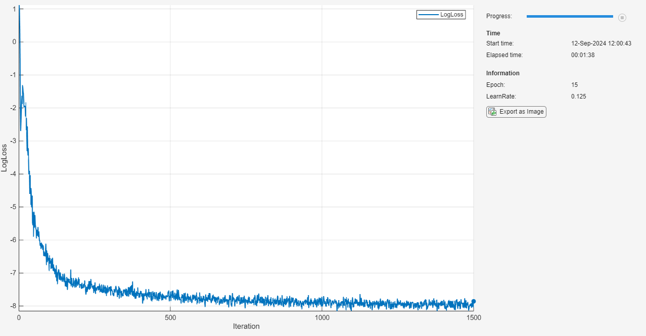
Initialize the TrainingProgressMonitor object. Because the timer starts when you create the monitor object, make sure that you create the object close to the training loop.
monitor = trainingProgressMonitor( ...
    Metrics="LogLoss", ...
    Info=["Epoch" "LearnRate"], ...
    XLabel="Iteration");
Train the network using a custom training loop. For each epoch, shuffle the data and loop over mini-batches of data. For each mini-batch:
Evaluate the model loss and gradients using the
dlfevalandmodelLossfunctions.Update the network parameters using the
sgdmupdatefunction.Display the training progress.
Stop if the
Stopproperty istrue. TheStopproperty value of theTrainingProgressMonitorobject changes to true when you click the Stop button.
Every learnRateDropPeriod epochs, multiply the learning rate by learnRateDropFactor.
epoch = 0;
iteration = 0;
learnRate = initialLearnRate;
start = tic;

% Loop over epochs.
while epoch < numEpochs  && ~monitor.Stop
    epoch = epoch + 1;

    % Shuffle data.
    mbq.shuffle

    % Loop over mini-batches.
    while hasdata(mbq) && ~monitor.Stop

        iteration = iteration + 1;

        % Read mini-batch of data.
        X = next(mbq);

        % Evaluate the model gradients and loss using dlfeval and the modelLoss function.
        [loss,gradients] = dlfeval(@modelLoss, net, X, icCoeff);

        % Update network parameters using the SGDM optimizer.
        [net,velocity] = sgdmupdate(net,gradients,velocity,learnRate,momentum);

        % Update the training progress monitor.
        recordMetrics(monitor,iteration,LogLoss=log(loss));
        updateInfo(monitor,Epoch=epoch,LearnRate=learnRate);
        monitor.Progress = 100 * iteration/numIterations;

    end

    % Reduce the learning rate.
    if mod(epoch,learnRateDropPeriod)==0
        learnRate = learnRate*learnRateDropFactor;
    end
end
Test Model
Test the accuracy of the network by comparing its predictions with the analytic solution.
Generate test data in the range to see if the network is able to extrapolate outside the training range .
xTest = linspace(0,4,1000)';
Make predictions using the minibatchpredict function. By default, the minibatchpredict function uses a GPU if one is available. Using a GPU requires a Parallel Computing Toolbox™ license and a supported GPU device. For information on supported devices, see GPU Computing Requirements (Parallel Computing Toolbox). Otherwise, the function uses the CPU. To specify the execution environment, use the ExecutionEnvironment option.
yModel = minibatchpredict(net,xTest);
Evaluate the analytic solution.
yAnalytic = exp(-xTest.^2);
Compare the analytic solution and the model prediction by plotting them on a logarithmic scale.
figure;
plot(xTest,yAnalytic,"-")
hold on
plot(xTest,yModel,"--")
legend("Analytic","Model")
xlabel("x")
ylabel("y (log scale)")
set(gca,YScale="log")
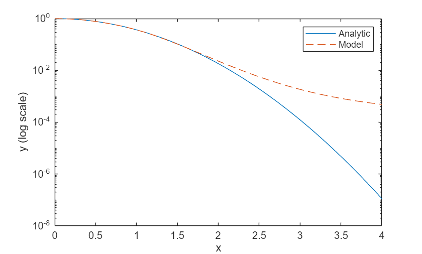
The model approximates the analytic solution accurately in the training range and it extrapolates in the range with lower accuracy.
Calculate the mean squared relative error in the training range .
yModelTrain = yModel(1:500);
yAnalyticTrain = yAnalytic(1:500);

errorTrain = mean(((yModelTrain-yAnalyticTrain)./yAnalyticTrain).^2)
errorTrain = single

0.0029
Calculate the mean squared relative error in the extrapolated range .
yModelExtra = yModel(501:1000);
yAnalyticExtra = yAnalytic(501:1000);

errorExtra = mean(((yModelExtra-yAnalyticExtra)./yAnalyticExtra).^2)
errorExtra = single

6.9634e+05
Notice that the mean squared relative error is higher in the extrapolated range than it is in the training range.
Model Loss Function
The modelLoss function takes as inputs a dlnetwork object net, a mini-batch of input data X, and the coefficient associated with the initial condition loss icCoeff. This function returns the gradients of the loss with respect to the learnable parameters in net and the corresponding loss. The loss is defined as a weighted sum of the ODE loss and the initial condition loss. The evaluation of this loss requires second order derivatives. To enable second order automatic differentiation, use the function dlgradient and set the EnableHigherDerivatives name-value argument to true.
function [loss,gradients] = modelLoss(net, X, icCoeff)
y = forward(net,X);

% Evaluate the gradient of y with respect to x.
% Since another derivative will be taken, set EnableHigherDerivatives to true.
dy = dlgradient(sum(y,"all"),X,EnableHigherDerivatives=true);

% Define ODE loss.
eq = dy + 2*y.*X;

% Define initial condition loss.
ic = forward(net,dlarray(0,"CB")) - 1;

% Specify the loss as a weighted sum of the ODE loss and the initial condition loss.
loss = mean(eq.^2,"all") + icCoeff * ic.^2;

% Evaluate model gradients.
gradients = dlgradient(loss, net.Learnables);

end
References
Maziar Raissi, Paris Perdikaris, and George Em Karniadakis, Physics Informed Deep Learning (Part I): Data-driven Solutions of Nonlinear Partial Differential Equations https://arxiv.org/abs/1711.10561
Lagaris, I. E., A. Likas, and D. I. Fotiadis. “Artificial Neural Networks for Solving Ordinary and Partial Differential Equations.” IEEE Transactions on Neural Networks 9, no. 5 (September 1998): 987–1000. https://doi.org/10.1109/72.712178.
See Also
dlarray | dlfeval | dlgradient