Compare Predictive Performance After Creating Models Using Econometric Modeler

This example shows how to choose lags for an ARIMA model by comparing the AIC values of estimated models using the Econometric Modeler app. The example also shows how to compare the predictive performance of several models that have the best in-sample fits at the command line. The data set Data_Airline.mat contains monthly counts of airline passengers.

Import Data into Econometric Modeler

At the command line, load the Data_Airline.mat data set.

load Data_Airline

To compare predictive performance later, reserve the last two years of data as a holdout sample.

fHorizon = 24;
HoldoutTimeTable = DataTimeTable((end - fHorizon + 1):end,:);
DataTimeTable((end - fHorizon + 1):end,:) = [];

At the command line, open the Econometric Modeler app.

econometricModeler

Alternatively, open the app from the apps gallery (see Econometric Modeler).

Import DataTimeTable into the app:

On the Econometric Modeler tab, in the Import section, click the Import button .
In the Import Data dialog box, in the Import? column, select the check box for the DataTimeTable variable.
Click Import.

The variable PSSG appears in the Time Series pane, its value appears in the Preview pane, and its time series plot appears in the Time Series Plot(PSSG) figure window.

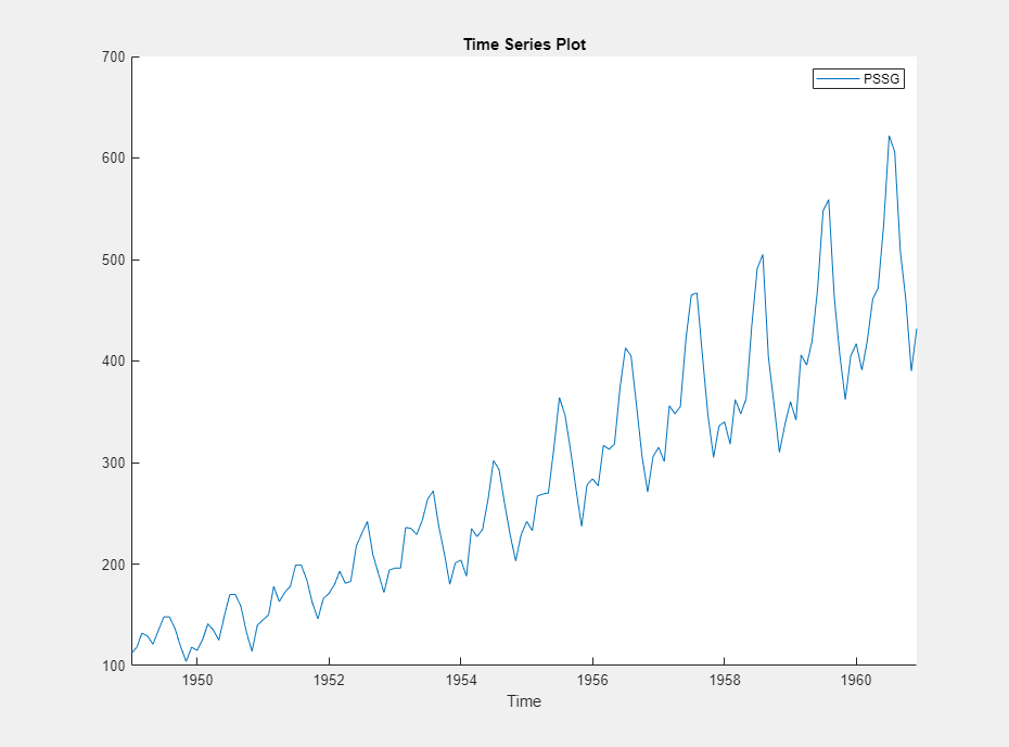
This screen shot shows a time series plot of the variable PSSG, with the x axis showing the time period of the late 1940's through the early 1960's.

The series exhibits a seasonal trend, serial correlation, and possible exponential growth. For an interactive analysis of serial correlation, see Detect Serial Correlation Using Econometric Modeler App.

Remove Exponential Trend

Address the exponential trend by applying the log transform to PSSG.

In the Time Series pane, select PSSG.
On the Econometric Modeler tab, in the Transforms section, click Log.

The transformed variable PSSGLog appears in the Time Series pane, its value appears in the Preview pane, and its time series plot appears in the Time Series Plot(PSSGLog) figure window.

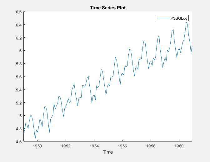
This screen shot shows a time series plot of PSSGLog, with the x axis showing the time period of the late 1940's through the early 1960's.

The exponential growth appears to be removed from the series.

Compare In-Sample Model Fits

Box, Jenkins, and Reinsel suggest a SARIMA(0,1,1)×(0,1,1)₁₂ model without a constant for PSSGLog [1] (for more details, see Estimate Multiplicative ARIMA Model Using Econometric Modeler App). However, consider all combinations of monthly SARIMA models that include up to two seasonal and nonseasonal MA lags. Specifically, iterate the following steps for each of the nine models of the form SARIMA(0,1,q)×(0,1,q₁₂)₁₂, where q ∈ {0,1,2} and q₁₂ ∈ {0,1,2}.

For the first iteration:
1. Let q = q₁₂ = 0.
2. With PSSGLog selected in the Time Series pane, click the Econometric Modeler tab. In the Models section, click the arrow to display the models gallery.
3. In the models gallery, in the ARMA/ARIMA Models section, click SARIMA.
4. In the SARIMA Model Parameters dialog box, on the Lag Order tab:
  - Nonseasonal section
    Set Degrees of Integration to 1.
    Set Moving Average Order to 0.
    Clear the Include Constant Term check box.
  - Seasonal section
    Set Period to 12 to indicate monthly data.
    Set Moving Average Order to 0.
    Select the Include Seasonal Difference check box.
5. Click Estimate.
Rename the new model variable.
1. In the Models pane, click the new model variable twice to select its name.
2. Enter SARIMA01qx01q₁₂. For example, when q = q₁₂ = 0, rename the variable to SARIMA010x010.
In the Model Summary(SARIMA01qx01q₁₂) document, in the Goodness of Fit table, note the AIC value. For example, for the model variable SARIMA010x010, the AIC is in this figure.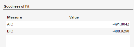
For the next iteration, choose values of q and q₁₂. For example, q = 0 and q₁₂ = 1 for the second iteration.
In the Models pane, right-click SARIMA01qx01q₁₂. In the context menu, select Modify to open the SARIMA Model Parameters dialog box with the current settings for the selected model.
In the SARIMA Model Parameters dialog box:
1. In the Nonseasonal section, set Moving Average Order to q.
2. In the Seasonal section, set Moving Average Order to q₁₂.
3. Click Estimate.

After you complete the steps, the Models pane contains nine estimated models named SARIMA010x010 through SARIMA012x012.

The resulting AIC values are in this table.

Model	Variable Name	AIC
SARIMA(0,1,0)×(0,1,0)₁₂	`SARIMA010x010`	-491.8042
SARIMA(0,1,0)×(0,1,1)₁₂	`SARIMA010x011`	-530.5327
SARIMA(0,1,0)×(0,1,2)₁₂	`SARIMA010x012`	-528.5330
SARIMA(0,1,1)×(0,1,0)₁₂	`SARIMA011x010`	-508.6853
SARIMA(0,1,1)×(0,1,1)₁₂	`SARIMA011x011`	-546.3970
SARIMA(0,1,1)×(0,1,2)₁₂	`SARIMA011x012`	-544.6444
SARIMA(0,1,2)×(0,1,0)₁₂	`SARIMA012x010`	-506.8027
SARIMA(0,1,2)×(0,1,1)₁₂	`SARIMA012x011`	-544.4789
SARIMA(0,1,2)×(0,1,2)₁₂	`SARIMA012x012`	-542.7171

The three models yielding the lowest three AIC values are SARIMA(0,1,1)×(0,1,1)₁₂, SARIMA(0,1,1)×(0,1,2)₁₂, and SARIMA(0,1,2)×(0,1,1)₁₂. These models have the best parsimonious in-sample fit.

Export Best Models to Workspace

Export the models with the best in-sample fits.

On the Econometric Modeler tab, in the Export section, click .
In the Export Variables dialog box, in the Models column, click the Select check box for the SARIMA011x011, SARIMA011x012, and SARIMA012x011. Clear the check box for any other selected models.
Click Export.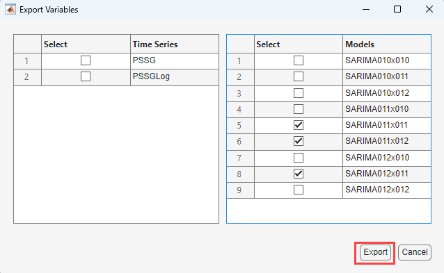

The arima model objects SARIMA011x011, SARIMA011x012, and SARIMA012x011 appear in the MATLAB^® Workspace.

Estimate Forecasts

At the command line, estimate two-year-ahead forecasts for each model.

f5 = forecast(SARIMA_PSSGLog5,fHorizon);
f6 = forecast(SARIMA_PSSGLog6,fHorizon);
f8 = forecast(SARIMA_PSSGLog8,fHorizon);

f5, f6, and f8 are 24-by-1 vectors containing the forecasts.

Compare Prediction Mean Square Errors

Estimate the prediction mean square error (PMSE) for each of the forecast vectors.

logPSSGHO = log(HoldoutTimeTable.Variables);
pmse5 = mean((logPSSGHO - f5).^2);
pmse6 = mean((logPSSGHO - f6).^2);
pmse8 = mean((logPSSGHO - f8).^2);

Identify the model yielding the lowest PMSE.

[~,bestIdx] = min([pmse5 pmse6 pmse8],[],2)

The SARIMA(0,1,1)×(0,1,1)₁₂ model performs the best in-sample and out-of-sample.

References

[1] Box, George E. P., Gwilym M. Jenkins, and Gregory C. Reinsel. Time Series Analysis: Forecasting and Control. 3rd ed. Englewood Cliffs, NJ: Prentice Hall, 1994.