estimate
Perform predictor variable selection for Bayesian linear regression models
Syntax
Description
PosteriorMdl = estimate(PriorMdl,X,y)estimate also performs predictor variable selection.
PriorMdl specifies the joint prior distribution of the parameters,
the structure of the linear regression model, and the variable selection algorithm.
X is the predictor data and y is the response
data. PriorMdl and PosteriorMdl are not the same
object type.
To produce PosteriorMdl, estimate updates the
prior distribution with information about the parameters that it obtains from the
data.
NaNs in the data indicate missing values, which
estimate removes using list-wise deletion.
PosteriorMdl = estimate(PriorMdl,X,y,Name,Value)'Lambda',0.5 specifies that the shrinkage parameter value for
Bayesian lasso regression is 0.5 for all coefficients except the
intercept.
If you specify Beta or Sigma2, then
PosteriorMdl and PriorMdl are equal.
[
uses any of the input argument combinations in the previous syntaxes and also returns a
table that includes the following for each parameter: posterior estimates, standard
errors, 95% credible intervals, and posterior probability that the parameter is greater
than 0.PosteriorMdl,Summary]
= estimate(___)
Examples
Consider the multiple linear regression model that predicts US real gross national product (GNPR) using a linear combination of industrial production index (IPI), total employment (E), and real wages (WR).
For all , is a series of independent Gaussian disturbances with a mean of 0 and variance .
Assume the prior distributions are:
For k = 0,...,3, has a Laplace distribution with a mean of 0 and a scale of , where is the shrinkage parameter. The coefficients are conditionally independent.
. and are the shape and scale, respectively, of an inverse gamma distribution.
Create a prior model for Bayesian lasso regression. Specify the number of predictors, the prior model type, and variable names. Specify these shrinkages:
0.01for the intercept10forIPIandWR1e5forEbecause it has a scale that is several orders of magnitude larger than the other variables
The order of the shrinkages follows the order of the specified variable names, but the first element is the shrinkage of the intercept.
p = 3;
PriorMdl = bayeslm(p,'ModelType','lasso','Lambda',[0.01; 10; 1e5; 10],...
    'VarNames',["IPI" "E" "WR"]);
PriorMdl is a lassoblm Bayesian linear regression model object representing the prior distribution of the regression coefficients and disturbance variance.
Load the Nelson-Plosser data set. Create variables for the response and predictor series.
load Data_NelsonPlosser
X = DataTable{:,PriorMdl.VarNames(2:end)};
y = DataTable{:,"GNPR"};
Perform Bayesian lasso regression by passing the prior model and data to estimate, that is, by estimating the posterior distribution of and . Bayesian lasso regression uses Markov chain Monte Carlo (MCMC) to sample from the posterior. For reproducibility, set a random seed.
rng(1);
PosteriorMdl = estimate(PriorMdl,X,y);
Method: lasso MCMC sampling with 10000 draws
Number of observations: 62
Number of predictors:   4

           |   Mean     Std           CI95        Positive  Distribution
-------------------------------------------------------------------------
 Intercept | -1.3472   6.8160  [-15.169, 11.590]    0.427     Empirical
 IPI       |  4.4755   0.1646   [ 4.157,  4.799]    1.000     Empirical
 E         |  0.0001   0.0002   [-0.000,  0.000]    0.796     Empirical
 WR        |  3.1610   0.3136   [ 2.538,  3.760]    1.000     Empirical
 Sigma2    | 60.1452  11.1180   [42.319, 85.085]    1.000     Empirical
PosteriorMdl is an empiricalblm model object that stores draws from the posterior distributions of and given the data. estimate displays a summary of the marginal posterior distributions in the MATLAB® command line. Rows of the summary correspond to regression coefficients and the disturbance variance, and columns correspond to characteristics of the posterior distribution. The characteristics include:
CI95, which contains the 95% Bayesian equitailed credible intervals for the parameters. For example, the posterior probability that the regression coefficient ofIPIis in [4.157, 4.799] is 0.95.Positive, which contains the posterior probability that the parameter is greater than 0. For example, the probability that the intercept is greater than 0 is0.427.
Plot the posterior distributions.
plot(PosteriorMdl)
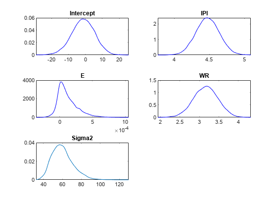
Given the shrinkages, the distribution of E is fairly dense around 0. Therefore, E might not be an important predictor.
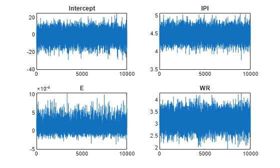
By default, estimate draws and discards a burn-in sample of size 5000. However, a good practice is to inspect a trace plot of the draws for adequate mixing and lack of transience. Plot a trace plot of the draws for each parameter. You can access the draws that compose the distribution (the properties BetaDraws and Sigma2Draws) using dot notation.
figure;
for j = 1:(p + 1)
    subplot(2,2,j);
    plot(PosteriorMdl.BetaDraws(j,:));
    title(sprintf('%s',PosteriorMdl.VarNames{j}));
end
figure;
plot(PosteriorMdl.Sigma2Draws);
title('Sigma2');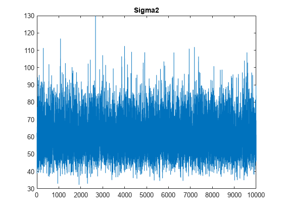
The trace plots indicate that the draws seem to mix well. The plots show no detectable transience or serial correlation, and the draws do not jump between states.
Consider the regression model in Select Variables Using Bayesian Lasso Regression.
Create a prior model for performing stochastic search variable selection (SSVS). Assume that and are dependent (a conjugate mixture model). Specify the number of predictors p and the names of the regression coefficients.
p = 3;
PriorMdl = mixconjugateblm(p,'VarNames',["IPI" "E" "WR"]);
Load the Nelson-Plosser data set. Create variables for the response and predictor series.
load Data_NelsonPlosser
X = DataTable{:,PriorMdl.VarNames(2:end)};
y = DataTable{:,'GNPR'};
Implement SSVS by estimating the marginal posterior distributions of and . Because SSVS uses Markov chain Monte Carlo for estimation, set a random number seed to reproduce the results.
rng(1);
PosteriorMdl = estimate(PriorMdl,X,y);
Method: MCMC sampling with 10000 draws
Number of observations: 62
Number of predictors:   4

           |   Mean      Std           CI95        Positive  Distribution  Regime
----------------------------------------------------------------------------------
 Intercept | -18.8333  10.1851  [-36.965,  0.716]    0.037     Empirical   0.8806
 IPI       |   4.4554   0.1543   [ 4.165,  4.764]    1.000     Empirical   0.4545
 E         |   0.0010   0.0004   [ 0.000,  0.002]    0.997     Empirical   0.0925
 WR        |   2.4686   0.3615   [ 1.766,  3.197]    1.000     Empirical   0.1734
 Sigma2    |  47.7557   8.6551   [33.858, 66.875]    1.000     Empirical    NaN
PosteriorMdl is an empiricalblm model object that stores draws from the posterior distributions of and given the data. estimate displays a summary of the marginal posterior distributions in the command line. Rows of the summary correspond to regression coefficients and the disturbance variance, and columns correspond to characteristics of the posterior distribution. The characteristics include:
CI95, which contains the 95% Bayesian equitailed credible intervals for the parameters. For example, the posterior probability that the regression coefficient ofE(standardized) is in [0.000, 0.0.002] is 0.95.Regime, which contains the marginal posterior probability of variable inclusion ( for a variable). For example, the posterior probabilityEthat should be included in the model is 0.0925.
Assuming that variables with Regime < 0.1 should be removed from the model, the results suggest that you can exclude the unemployment rate from the model.
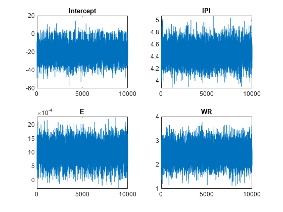
By default, estimate draws and discards a burn-in sample of size 5000. However, a good practice is to inspect a trace plot of the draws for adequate mixing and lack of transience. Plot a trace plot of the draws for each parameter. You can access the draws that compose the distribution (the properties BetaDraws and Sigma2Draws) using dot notation.
figure;
for j = 1:(p + 1)
    subplot(2,2,j);
    plot(PosteriorMdl.BetaDraws(j,:));
    title(sprintf('%s',PosteriorMdl.VarNames{j}));
end
figure;
plot(PosteriorMdl.Sigma2Draws);
title('Sigma2');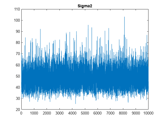
The trace plots indicate that the draws seem to mix well. The plots show no detectable transience or serial correlation, and the draws do not jump between states.
Consider the regression model and prior distribution in Select Variables Using Bayesian Lasso Regression.
Create a Bayesian lasso regression prior model for 3 predictors and specify variable names. Specify the shrinkage values 0.01, 10, 1e5, and 10 for the intercept, and the coefficients of IPI, E, and WR.
p = 3;
PriorMdl = bayeslm(p,'ModelType','lasso','VarNames',["IPI" "E" "WR"],...
    'Lambda',[0.01; 10; 1e5; 10]);
Load the Nelson-Plosser data set. Create variables for the response and predictor series.
load Data_NelsonPlosser
X = DataTable{:,PriorMdl.VarNames(2:end)};
y = DataTable{:,"GNPR"};
Estimate the conditional posterior distribution of given the data and that , and return the estimation summary table to access the estimates.
rng(1); % For reproducibility
[Mdl,SummaryBeta] = estimate(PriorMdl,X,y,'Sigma2',10);
Method: lasso MCMC sampling with 10000 draws
Conditional variable: Sigma2 fixed at  10
Number of observations: 62
Number of predictors:   4

           |   Mean     Std          CI95        Positive  Distribution
------------------------------------------------------------------------
 Intercept | -8.0643  4.1992  [-16.384,  0.018]    0.025     Empirical
 IPI       |  4.4454  0.0679   [ 4.312,  4.578]    1.000     Empirical
 E         |  0.0004  0.0002   [ 0.000,  0.001]    0.999     Empirical
 WR        |  2.9792  0.1672   [ 2.651,  3.305]    1.000     Empirical
 Sigma2    |   10      0       [10.000, 10.000]    1.000     Empirical
estimate displays a summary of the conditional posterior distribution of . Because is fixed at 10 during estimation, inferences on it are trivial.
Display Mdl.
Mdl
Mdl =
  lassoblm with properties:

    NumPredictors: 3
        Intercept: 1
         VarNames: {4×1 cell}
           Lambda: [4×1 double]
                A: 3
                B: 1


           |  Mean     Std           CI95         Positive   Distribution
---------------------------------------------------------------------------
 Intercept |  0       100    [-200.000, 200.000]    0.500   Scale mixture
 IPI       |  0      0.1000    [-0.200,  0.200]     0.500   Scale mixture
 E         |  0      0.0000    [-0.000,  0.000]     0.500   Scale mixture
 WR        |  0      0.1000    [-0.200,  0.200]     0.500   Scale mixture
 Sigma2    | 0.5000  0.5000    [ 0.138,  1.616]     1.000   IG(3.00,    1)
Because estimate computes the conditional posterior distribution, it returns the model input PriorMdl, not the conditional posterior, in the first position of the output argument list.
Display the estimation summary table.
SummaryBeta
SummaryBeta=5×6 table
                    Mean          Std                  CI95              Positive    Distribution                                   Covariances
                 __________    __________    ________________________    ________    _____________    _______________________________________________________________________

    Intercept       -8.0643        4.1992       -16.384       0.01837     0.0254     {'Empirical'}         17.633        0.17621    -0.00053724        0.11705              0
    IPI              4.4454      0.067949         4.312        4.5783          1     {'Empirical'}        0.17621      0.0046171    -1.4103e-06     -0.0068855              0
    E            0.00039896    0.00015673    9.4925e-05    0.00070697     0.9987     {'Empirical'}    -0.00053724    -1.4103e-06     2.4564e-08    -1.8168e-05              0
    WR               2.9792       0.16716        2.6506        3.3046          1     {'Empirical'}        0.11705     -0.0068855    -1.8168e-05       0.027943              0
    Sigma2               10             0            10            10          1     {'Empirical'}              0              0              0              0              0
SummaryBeta contains the conditional posterior estimates.
Estimate the conditional posterior distributions of given that is the conditional posterior mean of (stored in SummaryBeta.Mean(1:(end – 1))). Return the estimation summary table.
condPostMeanBeta = SummaryBeta.Mean(1:(end - 1));
[~,SummarySigma2] = estimate(PriorMdl,X,y,'Beta',condPostMeanBeta);
Method: lasso MCMC sampling with 10000 draws
Conditional variable: Beta fixed at -8.0643 4.4454 0.00039896 2.9792
Number of observations: 62
Number of predictors: 4
| Mean Std CI95 Positive Distribution
------------------------------------------------------------------------
Intercept | -8.0643 0.0000 [-8.064, -8.064] 0.000 Empirical
IPI | 4.4454 0.0000 [ 4.445, 4.445] 1.000 Empirical
E | 0.0004 0.0000 [ 0.000, 0.000] 1.000 Empirical
WR | 2.9792 0.0000 [ 2.979, 2.979] 1.000 Empirical
Sigma2 | 56.8314 10.2921 [39.947, 79.731] 1.000 Empirical
estimate displays an estimation summary of the conditional posterior distribution of given the data and that is condPostMeanBeta. In the display, inferences on are trivial.
Consider the regression model in Select Variables Using Bayesian Lasso Regression.
Create a prior model for performing SSVS. Assume that and are dependent (a conjugate mixture model). Specify the number of predictors p and the names of the regression coefficients.
p = 3;
PriorMdl = mixconjugateblm(p,'VarNames',["IPI" "E" "WR"]);
Load the Nelson-Plosser data set. Create variables for the response and predictor series.
load Data_NelsonPlosser
X = DataTable{:,PriorMdl.VarNames(2:end)};
y = DataTable{:,'GNPR'};
Implement SSVS by estimating the marginal posterior distributions of and . Because SSVS uses Markov chain Monte Carlo for estimation, set a random number seed to reproduce the results. Suppress the estimation display, but return the estimation summary table.
rng(1);
[PosteriorMdl,Summary] = estimate(PriorMdl,X,y,'Display',false);
PosteriorMdl is an empiricalblm model object that stores draws from the posterior distributions of and given the data. Summary is a table with columns corresponding to posterior characteristics and rows corresponding to the coefficients (PosteriorMdl.VarNames) and disturbance variance (Sigma2).
Display the estimated parameter covariance matrix (Covariances) and proportion of times the algorithm includes each predictor (Regime).
Covariances = Summary(:,"Covariances")Covariances=5×1 table
Covariances
______________________________________________________________________
Intercept 103.74 1.0486 -0.0031629 0.6791 7.3916
IPI 1.0486 0.023815 -1.3637e-05 -0.030387 0.06611
E -0.0031629 -1.3637e-05 1.3481e-07 -8.8792e-05 -0.00025044
WR 0.6791 -0.030387 -8.8792e-05 0.13066 0.089039
Sigma2 7.3916 0.06611 -0.00025044 0.089039 74.911
Regime = Summary(:,"Regime")Regime=5×1 table
Regime
______
Intercept 0.8806
IPI 0.4545
E 0.0925
WR 0.1734
Sigma2 NaN
Regime contains the marginal posterior probability of variable inclusion ( for a variable). For example, the posterior probability that E should be included in the model is 0.0925.
Assuming that variables with Regime < 0.1 should be removed from the model, the results suggest that you can exclude the unemployment rate from the model.
Input Arguments
Name-Value Arguments
Output Arguments
More About
Tips
Monte Carlo simulation is subject to variation. If
estimateuses Monte Carlo simulation, then estimates and inferences might vary when you callestimatemultiple times under seemingly equivalent conditions. To reproduce estimation results, before callingestimate, set a random number seed by usingrng.
Algorithms
This figure shows how estimate reduces the Monte Carlo sample
using the values of NumDraws, Thin, and
BurnIn.
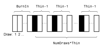
Rectangles represent successive draws from the distribution.
estimate removes the white rectangles from the Monte Carlo sample.
The remaining NumDraws black rectangles compose the Monte Carlo
sample.
Version History
Introduced in R2018b