Calibrating Hull-White Model Using Market Data

The pricing of interest-rate derivative securities relies on models that describe the underlying process. These interest rate models depend on one or more parameters that you must determine by matching the model predictions to the existing data available in the market. In the Hull-White model, there are two parameters related to the short rate process: mean reversion and volatility. Calibration is used to determine these parameters, such that the model can reproduce, as close as possible, the prices of caps or floors observed in the market. The calibration routines find the parameters that minimize the difference between the model price predictions and the market prices for caps and floors.

For a Hull-White model, the minimization is two dimensional, with respect to mean reversion (α) and volatility (σ). That is, calibrating the Hull-White model minimizes the difference between the model’s predicted prices and the observed market prices of the corresponding caplets or floorlets.

Hull-White Model Calibration Example

Use market data to identify the implied volatility (σ) and mean reversion (α) coefficients needed to build a Hull-White tree to price an instrument. The ideal case is to use the volatilities of the caps or floors used to calculate Alpha (α) and Sigma (σ). This will most likely not be the case, so market data must be interpolated to obtain the required values.

Consider a cap with these parameters:

Settle = ' Jan-21-2008';
Maturity = 'Mar-21-2011';
Strike = 0.0690;
Reset = 4;
Principal = 1000;
Basis = 0;

The caplets for this example would fall in:

capletDates = cfdates(Settle, Maturity, Reset, Basis);
datestr(capletDates')

ans =

21-Mar-2008
21-Jun-2008
21-Sep-2008
21-Dec-2008
21-Mar-2009
21-Jun-2009
21-Sep-2009
21-Dec-2009
21-Mar-2010
21-Jun-2010
21-Sep-2010
21-Dec-2010
21-Mar-2011

In the best case, look up the market volatilities for caplets with a Strike = 0.0690, and maturities in each reset date listed, but the likelihood of finding these exact instruments is low. As a consequence, use data that is available in the market and interpolate to find appropriate values for the caplets.

Based on the market data, you have the cap information for different dates and strikes. Assume that instead of having the data for Strike = 0.0690, you have the data for Strike1 = 0.0590 and Strike2 = 0.0790.

Maturity	Strike1 = 0.0590	Strike2 = 0.0790
21-Mar-2008	0.1533	0. 1526
21-Jun-2008	0.1731	0. 1730
21-Sep-2008	0. 1727	0. 1726
21-Dec-2008	0. 1752	0. 1747
21-Mar-2009	0. 1809	0. 1808
21-Jun-2009	0. 1809	0. 1792
21-Sep-2009	0. 1805	0. 1797
21-Dec-2009	0. 1802	0. 1794
21-Mar-2010	0. 1802	0. 1733
21-Jun-2010	0. 1757	0. 1751
21-Sep-2010	0. 1755	0. 1750
21-Dec-2010	0. 1755	0. 1745
21-Mar-2011	0. 1726	0. 1719

The nature of this data lends itself to matrix nomenclature, which is perfect for MATLAB^®. hwcalbycap requires that the dates, the strikes, and the actual volatility be separated into three variables: MarketStrike, MarketMat, and MarketVol.

MarketStrike = [0.0590; 0.0790];
MarketMat = {'21-Mar-2008';   
'21-Jun-2008'; 
'21-Sep-2008';  
'21-Dec-2008';  
'21-Mar-2009';  
'21-Jun-2009';  
'21-Sep-2009';  
'21-Dec-2009';  
'21-Mar-2010';  
'21-Jun-2010';  
'21-Sep-2010';  
'21-Dec-2010'; 
'21-Mar-2011'};


MarketVol = [0.1533 0.1731 0.1727 0.1752 0.1809 0.1800 0.1805 0.1802 0.1735 0.1757 ... 
             0.1755 0.1755 0.1726; % First row in table corresponding to Strike1 
             0.1526 0.1730 0.1726 0.1747 0.1808 0.1792 0.1797 0.1794 0.1733 0.1751 ... 
             0.1750 0.1745 0.1719]; % Second row in table corresponding to Strike2

Complete the input arguments using this data for RateSpec:

Rates = [0.0627;
0.0657;
0.0691;
0.0717;
0.0739;
0.0755;
0.0765;
0.0772;
0.0779;
0.0783;
0.0786;
0.0789;
0.0792;
0.0793];

ValuationDate = '21-Jan-2008';
EndDates = {'21-Mar-2008';'21-Jun-2008';'21-Sep-2008';'21-Dec-2008';...
            '21-Mar-2009';'21-Jun-2009';'21-Sep-2009';'21-Dec-2009';....
            '21-Mar-2010';'21-Jun-2010';'21-Sep-2010';'21-Dec-2010';....
            '21-Mar-2011';'21-Jun-2011'};
Compounding = 4;
Basis = 0;

RateSpec = intenvset('ValuationDate', ValuationDate, ...
'StartDates', ValuationDate, 'EndDates', EndDates, ...
'Rates', Rates, 'Compounding', Compounding, 'Basis', Basis)

RateSpec = 

           FinObj: 'RateSpec'
      Compounding: 4
             Disc: [14x1 double]
            Rates: [14x1 double]
         EndTimes: [14x1 double]
       StartTimes: [14x1 double]
         EndDates: [14x1 double]
       StartDates: 733428
    ValuationDate: 733428
            Basis: 0
     EndMonthRule: 1

Call the calibration routine to find values for volatility parameters Alpha and Sigma

Use hwcalbycap to calculate the values of Alpha and Sigma based on market data. Internally, hwcalbycap calls the function lsqnonlin. You can customize lsqnonlin by passing an optimization options structure created by optimoptions and then this can be passed to hwcalbycap using the name-value pair argument for OptimOptions. For example, optimoptions defines the target objective function tolerance as 100*eps and then calls hwcalbycap:

o=optimoptions('lsqnonlin','TolFun',100*eps);

[Alpha, Sigma] = hwcalbycap(RateSpec, MarketStrike, MarketMat, MarketVol,...
Strike, Settle, Maturity, 'Reset', Reset, 'Principal', Principal, 'Basis',... 
Basis, 'OptimOptions', o)

Local minimum possible.

lsqnonlin stopped because the size of the current step is less than
the default value of the step size tolerance.

Warning: LSQNONLIN did not converge to an optimal solution. It exited with exitflag = 2.
 
> In hwcalbycapfloor at 93
  In hwcalbycap at 75 

Alpha =

   1.0000e-06


Sigma =

    0.0127

The previous warning indicates that the conversion was not optimal. The search algorithm used by the Optimization Toolbox™ function lsqnonlin did not find a solution that conforms to all the constraints. To discern whether the solution is acceptable, look at the results of the optimization by specifying a third output (OptimOut) for hwcalbycap:

[Alpha, Sigma, OptimOut] = hwcalbycap(RateSpec, MarketStrike, MarketMat,...
MarketVol, Strike, Settle, Maturity, 'Reset', Reset, 'Principal', Principal,...
'Basis', Basis, 'OptimOptions', o);

The OptimOut.residual field of the OptimOut structure is the optimization residual. This value contains the difference between the Black caplets and those calculated during the optimization. You can use the OptimOut.residual value to calculate the percentual difference (error) compared to Black caplet prices and then decide whether the residual is acceptable. There is almost always some residual, so decide if it is acceptable to parameterize the market with a single value of Alpha and Sigma.

Price caplets using market data and Black's formula to obtain reference caplet values

To determine the effectiveness of the optimization, calculate reference caplet values using Black’s formula and the market data. Note, you must first interpolate the market data to obtain the caplets for calculation:

MarketMatNum = datenum(MarketMat);
[Mats, Strikes] = meshgrid(MarketMatNum, MarketStrike);
FlatVol = interp2(Mats, Strikes, MarketVol, datenum(Maturity), Strike, 'spline');

Compute the price of the cap using the Black model:

[CapPrice, Caplets] = capbyblk(RateSpec, Strike, Settle, Maturity, FlatVol,...
'Reset', Reset, 'Basis', Basis, 'Principal', Principal); 
Caplets = Caplets(2:end)';

Caplets =

    0.3210
    1.6355
    2.4863
    3.1903
    3.4110
    3.2685
    3.2385
    3.4803
    3.2419
    3.1949
    3.2991
    3.3750

Compare optimized values and Black values and display graphically

After calculating the reference values for the caplets, compare the values, analytically and graphically, to determine whether the calculated single values of Alpha and Sigma provide an adequate approximation:

OptimCaplets = Caplets+OptimOut.residual;

disp('   ');
disp('    Black76   Calibrated Caplets');
disp([Caplets                   OptimCaplets])

plot(MarketMatNum(2:end), Caplets, 'or', MarketMatNum(2:end), OptimCaplets, '*b');
datetick('x', 2)
xlabel('Caplet Maturity');
ylabel('Caplet Price');
title('Black and Calibrated Caplets');
h = legend('Black Caplets', 'Calibrated Caplets');
set(h, 'color', [0.9 0.9 0.9]);
set(h, 'Location', 'SouthEast');
set(gcf, 'NumberTitle', 'off')
grid on

 Black76   Calibrated Caplets
    0.3210    0.3636
    1.6355    1.6603
    2.4863    2.4974
    3.1903    3.1874
    3.4110    3.4040
    3.2685    3.2639
    3.2385    3.2364
    3.4803    3.4683
    3.2419    3.2408
    3.1949    3.1957
    3.2991    3.2960
    3.3750    3.3663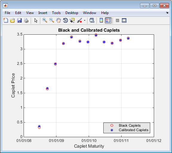

Compare cap prices using the Black, HW analytical, and HW tree models

Using the calculated caplet values, compare the prices of the corresponding cap using the Black model, Hull-White analytical, and Hull-White tree models. To calculate a Hull-White tree based on Alpha and Sigma, use these calibration routines:

• Black model:

  CapPriceBLK = CapPrice;

• HW analytical model:

  CapPriceHWAnalytical = sum(OptimCaplets);

• HW tree model to price the cap derived from the calibration process:

  1. Create VolSpec from the calibration parameters Alpha and Sigma:

     VolDates    = EndDates;
     VolCurve    = Sigma*ones(14,1);
     AlphaDates  = EndDates;
     AlphaCurve  = Alpha*ones(14,1);
     HWVolSpec = hwvolspec(ValuationDate, VolDates, VolCurve,AlphaDates, AlphaCurve);

  2. Create the TimeSpec:

     HWTimeSpec = hwtimespec(ValuationDate, EndDates, Compounding);

  3. Build the HW tree using the HW2000 method:

     HWTree = hwtree(HWVolSpec, RateSpec, HWTimeSpec, 'Method', 'HW2000');

  4. Price the cap:

     Price = capbyhw(HWTree, Strike, Settle, Maturity, Reset, Basis, Principal); 
     
     disp('   ');
     disp(['  CapPrice Black76 ..................:  ', num2str(CapPriceBLK,'%15.5f')]);
     disp(['  CapPrice HW analytical..........:  ', num2str(CapPriceHWAnalytical,'%15.5f')]);
     disp(['  CapPrice HW from capbyhw ..:  ', num2str(Price,'%15.5f')]);
     disp('   ');

     CapPrice Black76 ..........: 34.14220
     CapPrice HW analytical.....: 34.18008
     CapPrice HW from capbyhw ..: 34.14192

Price a portfolio of instruments using the calibrated HW tree

After building a Hull-White tree, based on parameters calibrated from market data, use HWTree to price a portfolio of these instruments:

• Two bonds

  CouponRate = [0.07; 0.09];
  Settle = ' Jan-21-2008';
  Maturity = {'Mar-21-2010';'Mar-21-2011'};
  Period = 1;
  Face = 1000;
  Basis = 0;
  

• Bond with an embedded American call option

  CouponRateOEB = 0.08;
  SettleOEB = ' Jan-21-2008';
  MaturityOEB = 'Mar-21-2011';
  OptSpec = 'call';
  StrikeOEB = 950;
  ExerciseDatesOEB = 'Mar-21-2011';
  AmericanOpt = 1;
  Period = 1;
  Face = 1000;
  Basis = 0;
  

To price this portfolio of instruments using the calibrated HWTree:

1. Use instadd to create the portfolio InstSet:

   InstSet = instadd('Bond', CouponRate, Settle,  Maturity, Period, Basis, [], [], [], [], [], Face);
   InstSet = instadd(InstSet,'OptEmBond',  CouponRateOEB, SettleOEB, MaturityOEB, OptSpec,...
   StrikeOEB,   ExerciseDatesOEB, 'AmericanOpt', AmericanOpt, 'Period', Period,...
   'Face',Face,  'Basis', Basis);
   

2. Add the cap instrument used in the calibration:

   SettleCap = ' Jan-21-2008';
   MaturityCap = 'Mar-21-2011';
   StrikeCap = 0.0690;
   Reset = 4;
   Principal = 1000;
   
   InstSet = instadd(InstSet,'Cap', StrikeCap, SettleCap, MaturityCap, Reset, Basis, Principal);

3. Assign names to the portfolio instruments:

   Names = {'7% Bond'; '8% Bond'; 'BondEmbCall'; '6.9% Cap'};
   InstSet = instsetfield(InstSet, 'Index',1:4, 'FieldName', {'Name'}, 'Data', Names );

4. Examine the set of instruments contained in InstSet:

   instdisp(InstSet)
   

   IdxType CoupRate Settle Mature Period Basis EOMRule IssueDate 1stCoupDate LastCoupDate StartDate Face Name
   
   1 Bond 0.07       21-Jan-2008    21-Mar-2010    1  0  NaN  NaN     NaN   NaN  NaN  1000    7% Bond
   2 Bond 0.09       21-Jan-2008    21-Mar-2011    1  0  NaN  NaN     NaN   NaN  NaN  1000    8% Bond
   
   IdxType CoupRate Settle Mature OptSpec Stke ExDate Per Basis EOMRule IssDate 1stCoupDate LstCoupDate StrtDate Face AmerOpt Name
   3 OptEmBond 0.08 21-Jan-2008 21-Mar-2011 call 950  21-Jan-2008  21-Mar-2011  1  0  1  NaN  NaN NaN  NaN  1000 1 BondEmbCall
    
   Index Type Strike Settle     Maturity   CapReset Basis Principal Name 
   4 Cap  0.069  21-Jan-2008    21-Mar-2011    4      0     1000    6.9% Cap   

5. Use hwprice to price the portfolio using the calibrated HWTree:

   format bank
   PricePortfolio = hwprice(HWTree, InstSet)

   PricePortfolio =
           980.45
          1023.05
           945.73
            34.14