Fuzzy C-Means Clustering for Iris Data
This example shows how to use fuzzy c-means clustering for the iris data set. This dataset was collected by botanist Edgar Anderson and contains random samples of flowers belonging to three species of iris flowers: setosa, versicolor, and virginica. For each of the species, the data set contains 50 observations for sepal length, sepal width, petal length, and petal width.
The example shows how to cluster data using Euclidean and Mahalanobis distance metrics and how to validate clustering results when you know the correct classification of the cluster training data.
Since R2026a: This example uses plotFuzzyClusters functionality introduced in R2026a. For a previous version of this example, see Fuzzy C-Means Clustering for Iris Data (R2025b).
Load Iris Data
Load the data set from the iris.dat data file.
iris = readmatrix("iris.dat");The iris matrix contains four columns of feature data and a fifth column that contains the index for the corresponding iris species.
Split the data into feature data and species index.
features = iris(:,1:4);
correctCluster = iris(:,5);
Find the logical index vector for each species.
setosaIndex = iris(:,5)==1;
versicolorIndex = iris(:,5)==2;
virginicaIndex = iris(:,5)==3;
Plot Data
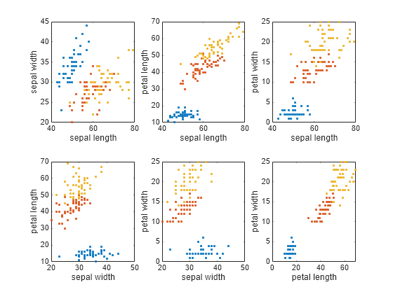
The iris data contains four dimensions representing sepal length, sepal width, petal length, and petal width. Plot the data points for each combination of two dimensions.
Define an array of feature names for labeling the plot axes.
featureNames = ["sepal length","sepal width","petal length","petal width"];
To plot the data clusters, first compute a crisp partition matrix for the correct species classification, where each data point has a membership value of 1 in its corresponding cluster and zero in the other clusters.
crispU = [setosaIndex';
          versicolorIndex';
          virginicaIndex'];
Plot the data clusters using the plotFuzzyClusters function and the crisp partition matrix. Since the plotting function requires a numeric partition matrix, convert the logical crispU matrix to a double matrix.
crispU = double(crispU);

figure(Position=[400 200 720 450])
plotFuzzyClusters(features,crispU, ...
    FeatureNames=featureNames, ...
    ShowMembershipPlot=false, ...
    Title="Correct Species Classification");
Configure Clustering Parameters
Specify the options for clustering the data using fuzzy c-means clustering with a default Euclidean distance metric.
NumClusters— Number of clusters. For this example, there are three clusters.Exponent— Fuzzy partition matrix exponent, which indicates the degree of fuzzy overlap between clusters. For more information, see Adjust Fuzzy Overlap in Fuzzy C-Means Clustering.MaxNumIteration— Maximum number of iterations. The clustering process stops after this number of iterations.MinImprovement— Minimum improvement. The clustering process stops when the objective function improvement between two consecutive iterations is less than this value.PartitionMatrix— Initial partition matrix containing cluster membership values for each data point. To compare between clustering results in this example, you use the same initial partition matrixinitUfor each clustering operation. Each column ofinitUcontains random membership values that sum to 1.
rng("default")
initU = rand(3,150);
initU = initU./sum(initU);

options = fcmOptions(...
    NumClusters=3,...
    Exponent=2.0, ...
    MaxNumIteration=1000, ...
    MinImprovement=1e-6, ...
    PartitionMatrix=initU);
For more information about these options and the fuzzy c-means algorithm, see fcm and fcmOptions.
Compute Clusters
Fuzzy c-means clustering is an iterative process. Initially, the fcm function either generates a random fuzzy partition matrix or uses the initial partition matrix that you provide. This matrix indicates the degree of membership of each data point in each cluster.
In each clustering iteration, fcm calculates the cluster centers and updates the fuzzy partition matrix using the calculated center locations. It then computes the objective function value based on the selected distance metric.
Cluster the data, displaying the objective function value after each iteration.
[centers,U] = fcm(features,options);
Iteration count = 1, obj. fcn = 28796.2
Iteration count = 2, obj. fcn = 20978.6
Iteration count = 3, obj. fcn = 15241.4
Iteration count = 4, obj. fcn = 11007.4
Iteration count = 5, obj. fcn = 10530.7
Iteration count = 6, obj. fcn = 10289.1
Iteration count = 7, obj. fcn = 9296.35
Iteration count = 8, obj. fcn = 7360.59
Iteration count = 9, obj. fcn = 6575.69
Iteration count = 10, obj. fcn = 6292.05
Iteration count = 11, obj. fcn = 6162.56
Iteration count = 12, obj. fcn = 6101.48
Iteration count = 13, obj. fcn = 6073.16
Iteration count = 14, obj. fcn = 6060.4
Iteration count = 15, obj. fcn = 6054.78
Iteration count = 16, obj. fcn = 6052.36
Iteration count = 17, obj. fcn = 6051.32
Iteration count = 18, obj. fcn = 6050.89
Iteration count = 19, obj. fcn = 6050.7
Iteration count = 20, obj. fcn = 6050.63
Iteration count = 21, obj. fcn = 6050.59
Iteration count = 22, obj. fcn = 6050.58
Iteration count = 23, obj. fcn = 6050.58
Iteration count = 24, obj. fcn = 6050.57
Iteration count = 25, obj. fcn = 6050.57
Iteration count = 26, obj. fcn = 6050.57
Iteration count = 27, obj. fcn = 6050.57
Iteration count = 28, obj. fcn = 6050.57
Iteration count = 29, obj. fcn = 6050.57
Iteration count = 30, obj. fcn = 6050.57
Iteration count = 31, obj. fcn = 6050.57
Iteration count = 32, obj. fcn = 6050.57
Iteration count = 33, obj. fcn = 6050.57
Minimum improvement reached.
The clustering stops when the objective function improvement is below the specified minimum threshold.
Since you supplied a random initial partition matrix, the cluster indices in computedCluster might not map correctly to the cluster indices in correctCluster. Using the reindexClusters helper function at the end of this example, reorder the clustering results.
[centers,U,reindexedCluster] = reindexClusters(centers,U,correctCluster);
Check the accuracy of the clustering results by first determining which data points are classified to the correct cluster.
clusterCorrect = (reindexedCluster == correctCluster);
Then, compute the percentage of correct classifications.
clusterAccuracy = round(100*sum(clusterCorrect)/length(clusterCorrect),1)
clusterAccuracy =
89.3000
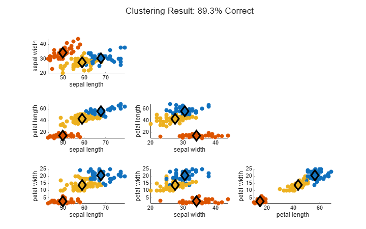
About 89% of the data points are clustered correctly.
Plot the clustering results.
figure(Position=[400 200 720 450])
plotFuzzyClusters(features,U,...
    ClusterCenters=centers, ...
    FeatureNames=featureNames, ...
    ShowMembershipPlot=false, ...
    Title="Clustering Result: "+clusterAccuracy+"% Correct");
Change Distance Metric
Since R2023a
By default, the fcm function uses a Euclidean distance metric when determining how far each data point is from each cluster center. This distance metric works best for spherical clusters.
Examining the data points, you can see that the iris clusters are not spherical. You can configure the fcm function to use a Mahalanobis distance metric, which generally works better for nonspherical clusters.
Cluster the data using a Mahalanobis distance metric and the same initial partition matrix.
options2 = fcmOptions(...
    NumClusters=3,...
    Exponent=2.0, ...
    MaxNumIteration=1000,...
    MinImprovement=1e-6, ...
    Verbose=false, ...
    PartitionMatrix=initU, ...
    DistanceMetric="mahalanobis");

[centers2,U2] = fcm(features,options2);
As with the first clustering operation, classify each data point to a cluster and reorder the computed clusters.
[centers2,U2,reindexedCluster2] = reindexClusters(centers2,U2,correctCluster);
Determine the accuracy of the new clustering results.
clusterCorrect2 = (reindexedCluster2 == correctCluster);
clusterAccuracy2 = round(100*sum(clusterCorrect2)/length(clusterCorrect2),1)
clusterAccuracy2 =
94.7000
Plot the new clustering results.
figure(Position=[400 200 720 450])
plotFuzzyClusters(features,U2,...
    ClusterCenters=centers2, ...
    FeatureNames=featureNames, ...
    ShowMembershipPlot=false, ...
    Title="Clustering Result: "+clusterAccuracy2+"% Correct");

Changing the distance metric has improved the clustering results to around 95%.
Local Functions
The reindexClusters function maps the computed clusters to the correct cluster indices in the original data using these steps:
Find the computed cluster indices by assigning each data point to the cluster for which it has a maximum membership value.
Determine which data points belong to each correct cluster.
Map the computed cluster indices to the correct cluster indices by finding the median computed cluster from the data points in a each correct cluster. This operation assumes that most data points are in a cluster with similar data points.
Reindex the computed clusters to use the correct cluster indices.
Reorder the computed cluster centers based on the mapping.
Reorder the rows of the partition matrix based on the mapping.
function [newCenters,newU,reindexedCluster] = reindexClusters(centers,U,correctClusters)

    % (1) Find computed cluster indices
    [~,computedClusters] = max(U);
    computedClusters = computedClusters';

    % (2) Determine which data points belong to each correct cluster.
    correctIndex1 = correctClusters==1;
    correctIndex2 = correctClusters==2;
    correctIndex3 = correctClusters==3;

    % (3) Map the computed cluster indices to the correct cluster indices.
    computedIndex = [median(computedClusters(correctIndex1));
                     median(computedClusters(correctIndex2));
                     median(computedClusters(correctIndex3))];

    % (4) Reindex the computed clusters.
    reindexedCluster = 1*(computedClusters==computedIndex(1)) + ...
                       2*(computedClusters==computedIndex(2)) + ...
                       3*(computedClusters==computedIndex(3));

    % (5) Reorder the computed cluster centers.
    newCenters = [centers(computedIndex==1,:);
                  centers(computedIndex==2,:);
                  centers(computedIndex==3,:)];

    % (6) Reorder the rows of the partition matrix.
    newU = [U(computedIndex==1,:);
            U(computedIndex==2,:);
            U(computedIndex==3,:)];
end