Point-Location Search

R2026b

A point-location search is a triangulation search algorithm that locates the simplex (triangle, tetrahedron, and so on) enclosing a query point. As in the case of the nearest-neighbor search, there are a few approaches to performing a point-location search in MATLAB, depending on the dimensionality of the problem:

• For 2-D and 3-D, use the class-based approach with the pointLocation method provided by the triangulation class and inherited by the delaunayTriangulation class.

• For 4-D and higher, use the delaunayn function to construct the triangulation and the complementary tsearchn function to perform the point-location search. Although supporting 2-D and 3-D, these N-D functions are not as general and efficient as the triangulation search methods.

2-D Triangulation Point-Location Search

Create a sample of 3-D points and compute the Voronoi vertices and diagram cells.

Load some 2-D data and plot a triangulation for the data set.

load trimesh2d
TR = triangulation(tri,x,y);
triplot(TR)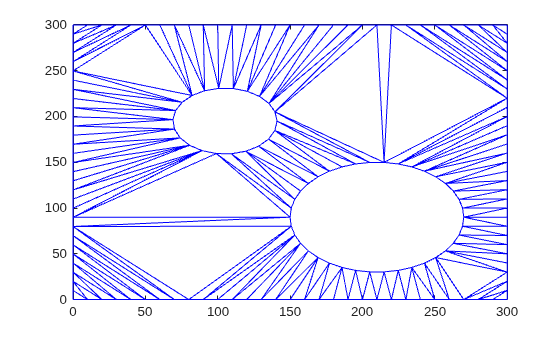

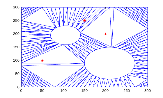
Create and add three query points to the triangulation plot.

hold on
Q = [50 100; 200 200; 150 250];
plot(Q(:,1),Q(:,2),"r*")

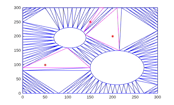
Find the indices of the corresponding enclosing triangles for the query points by using pointLocation. Use the indices to highlight the enclosing triangles in the plot.

pl = pointLocation(TR,Q);
triplot(TR.ConnectivityList(pl,:),TR.Points(:,1),TR.Points(:,2),"m")
hold off

2-D Delaunay Triangulation Point-Location Search

Begin with a set of 2-D points.

X = [3.5 8.2; 6.8 8.3; 1.3 6.5; 3.5 6.3; 5.8 6.2; ...
    8.3 6.5; 1 4; 2.7 4.3; 5 4.5; 7 3.5; 8.7 4.2; ...
    1.5 2.1; 4.1 1.1; 7 1.5; 8.5 2.75];

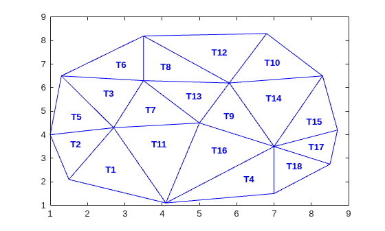
Create the triangulation and plot it showing the triangle ID labels at the incenters of the triangles.

dt = delaunayTriangulation(X);
triplot(dt);

hold on
ic = incenter(dt);
numtri = size(dt,1);
trilabels = arrayfun(@(x) {sprintf("T%d",x)},(1:numtri)');
Htl = text(ic(:,1), ic(:,2),trilabels,FontWeight="bold", ...
           HorizontalAlignment="center",Color="blue");

Now create some query points and add them to the plot.

q = [5.9344    6.2363;
    2.2143    2.1910;
    7.0948    3.6615;
    7.6040    2.2770;
    6.0724    2.5828;
    6.5464    6.9407;
    6.4588    6.1690;
    4.3534    3.9026;
    5.9329    7.7013;
    3.0271    2.2067];

plot(q(:,1),q(:,2),"*r"); 
vxlabels = arrayfun(@(n){sprintf("q%d",n)},(1:10)');
Hpl = text(q(:,1) + 0.2,q(:,2) + 0.2,vxlabels, ...
           FontWeight="bold", ...
           HorizontalAlignment="center", ...
           BackgroundColor="none");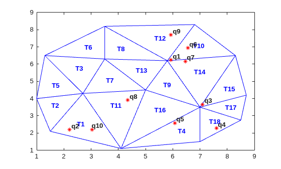

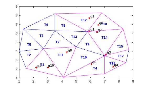
Find the indices of the corresponding enclosing triangles for the query points by using pointLocation. Use the indices to highlight the enclosing triangles in the plot.

ti = pointLocation(dt,q);
triplot(dt.ConnectivityList(ti,:),dt.Points(:,1),dt.Points(:,2),"m")
hold off

3-D and 4-D Delaunay Triangulation Point-Location Search

Performing a point-location search in 3-D is a direct extension of performing a point-location search in 2-D with delaunayTriangulation.

For 4-D and higher, use the delaunayn and tsearchn functions as illustrated in the following example:

Create a random sample of points in 4-D and triangulate them using delaunayn:

X = 20*rand(50,4) - 10;
tri = delaunayn(X);

Create some query points and find the index of the corresponding enclosing simplices using the tsearchn function:

q = rand(5,4);
ti = tsearchn(X,tri,q);

The pointLocation method and the tsearchn function allow the corresponding barycentric coordinates to be returned as an optional argument. In the 4-D example, you can compute the barycentric coordinates as follows:

[ti,bc] = tsearchn(X,tri,q);

The barycentric coordinates are useful for performing linear interpolation. These coordinates provide you with weights that you can use to scale the values at each vertex of the enclosing simplex. See Interpolating Scattered Data for further details.