Solve BVP with Two Solutions

This example uses bvp4c with two different initial guesses to find both solutions to a BVP problem.

Consider the differential equation

${{\mathit{y}}^{\prime }}^{\prime }+{\mathit{e}}^{\mathit{y}}=0$.

This equation is subject to the boundary conditions

$\mathit{y}\left(0\right)=\mathit{y}\left(1\right)=0$.

To solve this equation in MATLAB®, you need to code the equation and boundary conditions, then generate a suitable initial guess for the solution before calling the boundary value problem solver bvp4c. You either can include the required functions as local functions at the end of a file (as done here), or save them as separate, named files in a directory on the MATLAB path.

Code Equation

Create a function to code the equation. This function should have the signature dydx = bvpfun(x,y) or dydx = bvpfun(x,y,parameters), where:

• x is the independent variable.

• y is the solution (dependent variable).

• parameters is a vector of unknown parameter values (optional).

These inputs are automatically passed to the function by the solver, but the variable names determine how you code the equations. In this case, you can rewrite the second-order equation as a system of first-order equations

${{\mathit{y}}_1}^{\prime }={\mathit{y}}_2$,

${{\mathit{y}}_2}^{\prime }=-{\mathit{e}}^{{\mathit{y}}_1}$.

The function encoding these equations is

function dydx = bvpfun(x,y)
dydx = [y(2)
        -exp(y(1))];
end

Code Boundary Conditions

For two-point boundary value conditions like the ones in this problem, the boundary conditions function should have the signature res = bcfun(ya,yb) or res = bcfun(ya,yb,parameters), depending on whether unknown parameters are involved. ya and yb are column vectors that the solver automatically passes to the function, and bcfun returns the residual in the boundary conditions.

For the boundary conditions $\mathit{y}\left(0\right)=\mathit{y}\left(1\right)=0$, the bcfun function specifies that the residual value is zero at both boundaries. These residual values are enforced at the first and last points of the mesh that you specify to bvpinit in your initial guess. The initial mesh in this problem should have x(1) = 0 and x(end) = 1.

function res = bcfun(ya,yb)
res = [ya(1)
       yb(1)];
end

Form Initial Guess

Call bvpinit to generate an initial guess of the solution. The mesh for x does not need to have a lot of points, but the first point must be 0. Then the last point must be 1 so that the boundary conditions are properly specified. Use an initial guess for y where the first component is slightly positive and the second component is zero.

xmesh = linspace(0,1,5);
solinit = bvpinit(xmesh, [0.1 0]);

Solve Equation

Solve the BVP using the bvp4c solver.

sol1 = bvp4c(@bvpfun, @bcfun, solinit);

Use Different Initial Guess

Solve the BVP a second time using a different initial guess for the solution.

solinit = bvpinit(xmesh, [3 0]);
sol2 = bvp4c(@bvpfun, @bcfun, solinit);

Compare Solutions

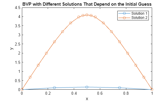
Plot the solutions that bvp4c calculates for the different initial conditions. Both solutions satisfy the stated boundary conditions, but have different behaviors inbetween. Since the solution is not always unique, the different behaviors show the importance of giving a good initial guess for the solution.

plot(sol1.x,sol1.y(1,:),'-o',sol2.x,sol2.y(1,:),'-o')
title('BVP with Different Solutions That Depend on the Initial Guess')
xlabel('x')
ylabel('y')
legend('Solution 1','Solution 2')

Local Functions

Listed here are the local helper functions that the BVP solver bvp4c calls to calculate the solution. Alternatively, you can save these functions as their own files in a directory on the MATLAB path.

function dydx = bvpfun(x,y) % equation being solved
dydx = [y(2)
        -exp(y(1))];
end
%-------------------------------------------
function res = bcfun(ya,yb) % boundary conditions 
res = [ya(1)
       yb(1)];
end
%-------------------------------------------