histogram2
Bivariate histogram plot
Description
Bivariate histograms are a type of bar plot for numeric data that group the
data into 2-D bins. After you create a Histogram2 object, you can
modify aspects of the histogram by changing its property values. This is particularly
useful for quickly modifying the properties of the bins or changing the
display.
Creation
Syntax
Description
histogram2( creates a
bivariate histogram plot of X,Y)X and Y.
The histogram2 function uses an automatic binning
algorithm that returns bins with a uniform area, chosen to cover the range
of elements in X and Y and reveal the
underlying shape of the distribution. histogram2
displays the bins as 3-D rectangular bars such that the height of each bar
indicates the number of elements in the bin.
histogram2(___,
specifies additional parameters using one or more name-value arguments for
any of the previous syntaxes. For example, specify
Name,Value)Normalization to use a different type of
normalization. For a list of properties, see Histogram2 Properties.
histogram2(
plots into the specified axes instead of into the current axes
(ax,___)gca). ax can precede any of the
input argument combinations in the previous syntaxes.
h = histogram2(___)Histogram2 object. Use this to inspect and
adjust properties of the bivariate histogram. For a list of properties, see
Histogram2 Properties.
Input Arguments
Name-Value Arguments
Specify optional pairs of arguments as
Name1=Value1,...,NameN=ValueN, where Name is
the argument name and Value is the corresponding value.
Name-value arguments must appear after other arguments, but the order of the
pairs does not matter.
Example: histogram2(X,Y,BinWidth=[5 10])
Before R2021a, use commas to separate each name and value, and enclose
Name in quotes.
Example: histogram2(X,Y,'BinWidth',[5 10])
Note
The properties listed here are only a subset. For a complete list, see Histogram2 Properties.
Bins
Data
Color and Styling
Histogram display style, specified as either 'bar3' or
'tile'.
'bar3'— Display the histogram using 3-D bars.'tile'— Display the histogram as a rectangular array of tiles with colors indicating the bin values.
Example: histogram2(X,Y,'DisplayStyle','tile') plots the histogram
as a rectangular array of tiles.
Histogram bar color, specified as one of these values:
'none'— Bars are not filled.'flat'— Bar colors vary with height. Bars with different heights have different colors. The colors are selected from the figure or axes colormap.'auto'— Histogram bar color is chosen automatically (default).RGB triplet, hexadecimal color code, or color name — Bars are filled with the specified color.
RGB triplets and hexadecimal color codes are useful for specifying custom colors.
An RGB triplet is a three-element row vector whose elements specify the intensities of the red, green, and blue components of the color. The intensities must be in the range
[0,1]; for example,[0.4 0.6 0.7].A hexadecimal color code is a character vector or a string scalar that starts with a hash symbol (
#) followed by three or six hexadecimal digits, which can range from0toF. The values are not case sensitive. Thus, the color codes"#FF8800","#ff8800","#F80", and"#f80"are equivalent.
Alternatively, you can specify some common colors by name. This table lists the named color options, the equivalent RGB triplets, and hexadecimal color codes.
Color Name Short Name RGB Triplet Hexadecimal Color Code Appearance "red""r"[1 0 0]"#FF0000"
"green""g"[0 1 0]"#00FF00"
"blue""b"[0 0 1]"#0000FF"
"cyan""c"[0 1 1]"#00FFFF"
"magenta""m"[1 0 1]"#FF00FF"
"yellow""y"[1 1 0]"#FFFF00"
"black""k"[0 0 0]"#000000"
"white""w"[1 1 1]"#FFFFFF"
This table lists the default color palettes for plots in the light and dark themes.
Palette Palette Colors "gem"— Light theme defaultBefore R2025a: Most plots use these colors by default.

"glow"— Dark theme default
You can get the RGB triplets and hexadecimal color codes for these palettes using the
orderedcolorsandrgb2hexfunctions. For example, get the RGB triplets for the"gem"palette and convert them to hexadecimal color codes.RGB = orderedcolors("gem"); H = rgb2hex(RGB);Before R2023b: Get the RGB triplets using
RGB = get(groot,"FactoryAxesColorOrder").Before R2024a: Get the hexadecimal color codes using
H =
            compose("#%02X%02X%02X",round(RGB*255))
.
If you specify DisplayStyle as 'tile', then the
FaceColor property is set to 'flat'.
Example: histogram2(X,Y,'FaceColor','g')
Histogram edge color, specified as one of these values:
'none'— Edges are not drawn.'auto'— Color of each edge is chosen automatically.RGB triplet, hexadecimal color code, or color name — Edges use the specified color.
RGB triplets and hexadecimal color codes are useful for specifying custom colors.
An RGB triplet is a three-element row vector whose elements specify the intensities of the red, green, and blue components of the color. The intensities must be in the range
[0,1]; for example,[0.4 0.6 0.7].A hexadecimal color code is a character vector or a string scalar that starts with a hash symbol (
#) followed by three or six hexadecimal digits, which can range from0toF. The values are not case sensitive. Thus, the color codes"#FF8800","#ff8800","#F80", and"#f80"are equivalent.
Alternatively, you can specify some common colors by name. This table lists the named color options, the equivalent RGB triplets, and hexadecimal color codes.
Color Name Short Name RGB Triplet Hexadecimal Color Code Appearance "red""r"[1 0 0]"#FF0000""green""g"[0 1 0]"#00FF00""blue""b"[0 0 1]"#0000FF""cyan""c"[0 1 1]"#00FFFF""magenta""m"[1 0 1]"#FF00FF""yellow""y"[1 1 0]"#FFFF00""black""k"[0 0 0]"#000000""white""w"[1 1 1]"#FFFFFF"This table lists the default color palettes for plots in the light and dark themes.
Palette Palette Colors "gem"— Light theme defaultBefore R2025a: Most plots use these colors by default.
"glow"— Dark theme defaultYou can get the RGB triplets and hexadecimal color codes for these palettes using the
orderedcolorsandrgb2hexfunctions. For example, get the RGB triplets for the"gem"palette and convert them to hexadecimal color codes.RGB = orderedcolors("gem"); H = rgb2hex(RGB);Before R2023b: Get the RGB triplets using
RGB = get(groot,"FactoryAxesColorOrder").Before R2024a: Get the hexadecimal color codes using
H =
            compose("#%02X%02X%02X",round(RGB*255))
.
Example: histogram2(X,Y,'EdgeColor','r')
Lighting effect on histogram bars, specified as one of these values.
| Value | Description |
|---|---|
'lit' |
Histogram bars display a pseudo-lighting effect, where the sides of the bars use darker colors relative to the tops. The bars are unaffected by other light sources in the axes. This is the default value when |
'flat' |
Histogram bars are not lit automatically. In the presence of other light objects, the lighting effect is uniform across the bar faces. |
'none' |
Histogram bars are not lit automatically, and lights do not affect the histogram bars.
|
Example: histogram2(X,Y,'FaceLighting','none') turns off the
lighting of the histogram bars.
Line style, specified as one of the options listed in this table.
| Line Style | Description | Resulting Line |
|---|---|---|
"-" | Solid line |
|
"--" | Dashed line |
|
":" | Dotted line |
|
"-." | Dash-dotted line |
|
"none" | No line | No line |
Output Arguments
Properties
| Histogram2 Properties | Bivariate histogram appearance and behavior |
Examples
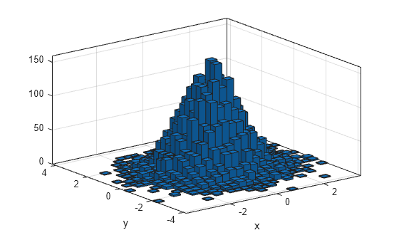
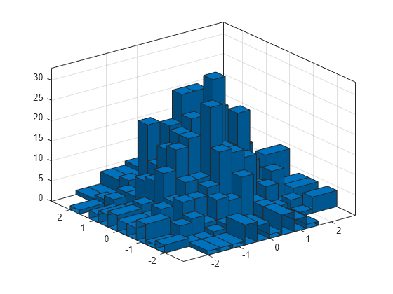
Generate 10,000 pairs of random numbers and create a bivariate histogram. The histogram2 function automatically chooses an appropriate number of bins to cover the range of values in x and y and show the shape of the underlying distribution.
x = randn(10000,1);
y = randn(10000,1);
h = histogram2(x,y)
h =
  Histogram2 with properties:

             Data: [10000×2 double]
           Values: [25×28 double]
          NumBins: [25 28]
        XBinEdges: [-3.9000 -3.6000 -3.3000 -3 -2.7000 -2.4000 -2.1000 -1.8000 -1.5000 -1.2000 -0.9000 -0.6000 -0.3000 0 0.3000 0.6000 0.9000 1.2000 1.5000 1.8000 2.1000 2.4000 2.7000 3.0000 3.3000 3.6000]
        YBinEdges: [-4.2000 -3.9000 -3.6000 -3.3000 -3.0000 -2.7000 -2.4000 -2.1000 -1.8000 -1.5000 -1.2000 -0.9000 -0.6000 -0.3000 0 0.3000 0.6000 0.9000 1.2000 1.5000 1.8000 2.1000 2.4000 2.7000 3 3.3000 3.6000 3.9000 4.2000]
         BinWidth: [0.3000 0.3000]
    Normalization: 'count'
        FaceColor: 'auto'
        EdgeColor: [0.1294 0.1294 0.1294]

  Show all properties
xlabel('x')
ylabel('y')
When you specify an output argument to the histogram2 function, it returns a histogram2 object. You can use this object to inspect the properties of the histogram, such as the number of bins or the width of the bins.
Find the number of histogram bins in each dimension.
nXnY = h.NumBins
nXnY = 1×2

    25    28
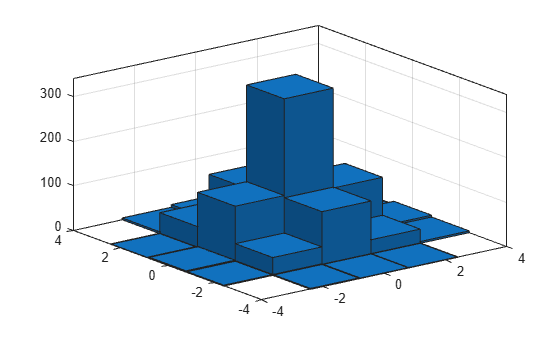
Plot a bivariate histogram of 1,000 pairs of random numbers sorted into 25 equally spaced bins, using 5 bins in each dimension.
x = randn(1000,1);
y = randn(1000,1);
nbins = 5;
h = histogram2(x,y,nbins)
h =
  Histogram2 with properties:

             Data: [1000×2 double]
           Values: [5×5 double]
          NumBins: [5 5]
        XBinEdges: [-4 -2.4000 -0.8000 0.8000 2.4000 4]
        YBinEdges: [-4 -2.4000 -0.8000 0.8000 2.4000 4]
         BinWidth: [1.6000 1.6000]
    Normalization: 'count'
        FaceColor: 'auto'
        EdgeColor: [0.1294 0.1294 0.1294]

  Show all properties
Find the resulting bin counts.
counts = h.Values
counts = 5×5

     0     2     3     1     0
     2    40   124    47     4
     1   119   341   109    10
     1    32   117    33     1
     0     4     8     1     0
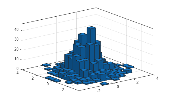
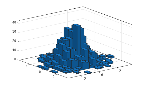
Generate 1,000 pairs of random numbers and create a bivariate histogram.
x = randn(1000,1);
y = randn(1000,1);
h = histogram2(x,y)
h =
  Histogram2 with properties:

             Data: [1000×2 double]
           Values: [15×15 double]
          NumBins: [15 15]
        XBinEdges: [-3.5000 -3 -2.5000 -2 -1.5000 -1 -0.5000 0 0.5000 1 1.5000 2 2.5000 3 3.5000 4]
        YBinEdges: [-3.5000 -3 -2.5000 -2 -1.5000 -1 -0.5000 0 0.5000 1 1.5000 2 2.5000 3 3.5000 4]
         BinWidth: [0.5000 0.5000]
    Normalization: 'count'
        FaceColor: 'auto'
        EdgeColor: [0.1294 0.1294 0.1294]

  Show all properties
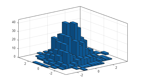
Use the morebins function to coarsely adjust the number of bins in the x dimension.
nbins = morebins(h,'x');
nbins = morebins(h,'x')
nbins = 1×2

    19    15
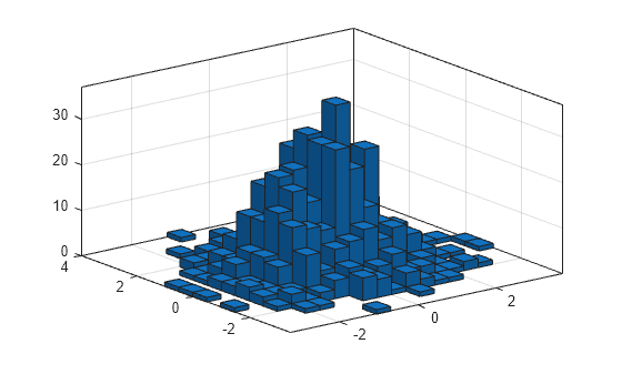
Use the fewerbins function to adjust the number of bins in the y dimension.
nbins = fewerbins(h,'y');
nbins = fewerbins(h,'y')
nbins = 1×2

    19    11
Adjust the number of bins at a fine grain level by explicitly setting the number of bins.
h.NumBins = [20 10];
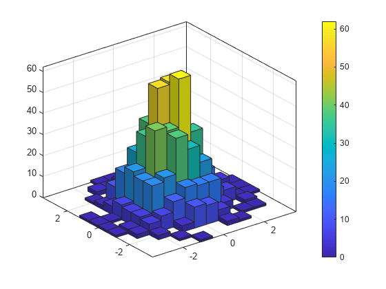
Create a bivariate histogram using 1,000 normally distributed random numbers with 12 bins in each dimension. Specify FaceColor as 'flat' to color the histogram bars by height.
h = histogram2(randn(1000,1),randn(1000,1),[12 12],'FaceColor','flat');
colorbar
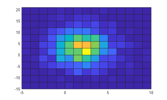
Generate random data and plot a bivariate tiled histogram. Display the empty bins by specifying ShowEmptyBins as 'on'.
x = 2*randn(1000,1)+2;
y = 5*randn(1000,1)+3;
h = histogram2(x,y,'DisplayStyle','tile','ShowEmptyBins','on');
Generate 1,000 pairs of random numbers and create a bivariate histogram. Specify the bin edges using two vectors, with infinitely wide bins on the boundary of the histogram to capture all outliers that do not satisfy .
x = randn(1000,1);
y = randn(1000,1);
Xedges = [-Inf -2:0.4:2 Inf];
Yedges = [-Inf -2:0.4:2 Inf];
h = histogram2(x,y,Xedges,Yedges)
h =
  Histogram2 with properties:

             Data: [1000×2 double]
           Values: [12×12 double]
          NumBins: [12 12]
        XBinEdges: [-Inf -2 -1.6000 -1.2000 -0.8000 -0.4000 0 0.4000 0.8000 1.2000 1.6000 2 Inf]
        YBinEdges: [-Inf -2 -1.6000 -1.2000 -0.8000 -0.4000 0 0.4000 0.8000 1.2000 1.6000 2 Inf]
         BinWidth: 'nonuniform'
    Normalization: 'count'
        FaceColor: 'auto'
        EdgeColor: [0.1294 0.1294 0.1294]

  Show all properties
When the bin edges are infinite, histogram2 displays each outlier bin (along the boundary of the histogram) as being double the width of the bin next to it.
Specify the Normalization property as 'countdensity' to remove the bins containing the outliers. Now the volume of each bin represents the frequency of observations in that interval.
h.Normalization = 'countdensity';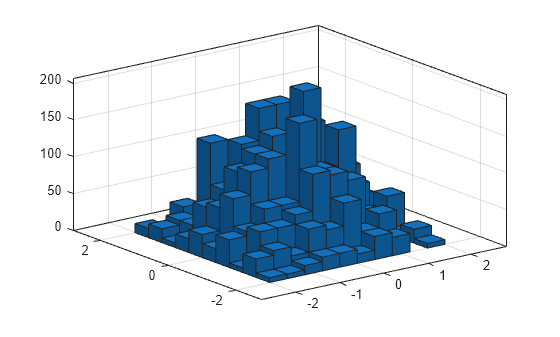
Generate 1,000 pairs of random numbers and create a bivariate histogram using the 'probability' normalization.
x = randn(1000,1);
y = randn(1000,1);
h = histogram2(x,y,'Normalization','probability')

h =
  Histogram2 with properties:

             Data: [1000×2 double]
           Values: [15×15 double]
          NumBins: [15 15]
        XBinEdges: [-3.5000 -3 -2.5000 -2 -1.5000 -1 -0.5000 0 0.5000 1 1.5000 2 2.5000 3 3.5000 4]
        YBinEdges: [-3.5000 -3 -2.5000 -2 -1.5000 -1 -0.5000 0 0.5000 1 1.5000 2 2.5000 3 3.5000 4]
         BinWidth: [0.5000 0.5000]
    Normalization: 'probability'
        FaceColor: 'auto'
        EdgeColor: [0.1294 0.1294 0.1294]

  Show all properties
Compute the total sum of the bar heights. With this normalization, the height of each bar is equal to the probability of selecting an observation within that bin interval, and the heights of all of the bars sum to 1.
S = sum(h.Values(:))
S =
1
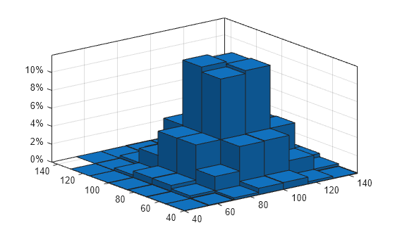
Generate 100,000 normally distributed random vectors. Use a standard deviation of 15 and means of 100 and 85.
x = [100 85] + 15*randn(1e5,2);
Plot a histogram of the random vectors. Scale and label the z-axis as percentages.
edges = 40:15:145;
histogram2(x(:,1),x(:,2),edges,edges,Normalization="percentage")
ztickformat("percentage")
Generate 1,000 pairs of random numbers and create a bivariate histogram. Return the histogram object to adjust the properties of the histogram without recreating the entire plot.
x = randn(1000,1);
y = randn(1000,1);
h = histogram2(x,y)

h =
  Histogram2 with properties:

             Data: [1000×2 double]
           Values: [15×15 double]
          NumBins: [15 15]
        XBinEdges: [-3.5000 -3 -2.5000 -2 -1.5000 -1 -0.5000 0 0.5000 1 1.5000 2 2.5000 3 3.5000 4]
        YBinEdges: [-3.5000 -3 -2.5000 -2 -1.5000 -1 -0.5000 0 0.5000 1 1.5000 2 2.5000 3 3.5000 4]
         BinWidth: [0.5000 0.5000]
    Normalization: 'count'
        FaceColor: 'auto'
        EdgeColor: [0.1294 0.1294 0.1294]

  Show all properties
Color the histogram bars by height.
h.FaceColor = 'flat';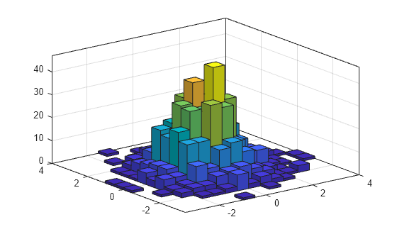
Change the number of bins in each direction.
h.NumBins = [10 25];

Display the histogram as a tile plot.
h.DisplayStyle = 'tile';
view(2)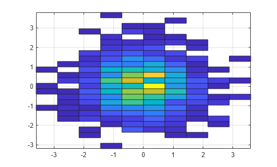
Use the savefig function to save a histogram2 figure.
histogram2(randn(100,1),randn(100,1));
savefig('histogram2.fig');
close gcf
Use openfig to load the histogram figure back into MATLAB®. openfig also returns a handle to the figure, h.
h = openfig('histogram2.fig');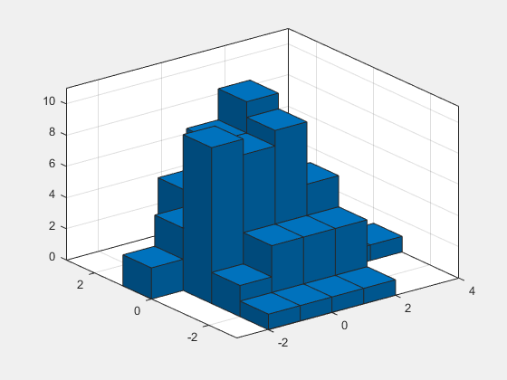
Use the findobj function to locate the correct object handle from the figure handle. This allows you to continue manipulating the original histogram object used to generate the figure.
y = findobj(h,'type','histogram2')
y =
  Histogram2 with properties:

             Data: [100×2 double]
           Values: [7×6 double]
          NumBins: [7 6]
        XBinEdges: [-3 -2 -1 0 1 2 3 4]
        YBinEdges: [-3 -2 -1 0 1 2 3]
         BinWidth: [1 1]
    Normalization: 'count'
        FaceColor: 'auto'
        EdgeColor: [0.1294 0.1294 0.1294]

  Show all properties
Tips
Histogram plots created using
histogram2have a context menu in plot edit mode that enables interactive manipulations in the figure window. For example, you can use the context menu to interactively change the number of bins, align multiple histograms, or change the display order.
Extended Capabilities
Version History
Introduced in R2015bSee Also
Histogram2 Properties | bar3 | discretize | fewerbins | morebins | histcounts2 | histcounts