semilogx
Semilog plot (x-axis has log scale)
Syntax
Description
Vector and Matrix Data
semilogx( plots
x- and y-coordinates using a base-10 logarithmic
scale on the x-axis and a linear scale on the y-axis.X,Y)
To plot a set of coordinates connected by line segments, specify
XandYas vectors of the same length.To plot multiple sets of coordinates on the same set of axes, specify at least one of
XorYas a matrix.
semilogx( plots Y)Y
against an implicit set of x-coordinates.
If
Yis a vector, the x-coordinates range from 1 tolength(Y).If
Yis a matrix, the plot contains one line for each column inY. The x-coordinates range from 1 to the number of rows inY.
If Y contains complex numbers,
semilogx plots the imaginary part of Y versus
the real part of Y. However, if you specify both X
and Y, MATLAB® ignores the imaginary part.
Table Data
semilogx(
plots the variables tbl,xvar,yvar)xvar and yvar from the table
tbl. To plot one data set, specify one variable for
xvar and one variable for yvar. To plot multiple
data sets, specify multiple variables for xvar,
yvar, or both. If both arguments specify multiple variables, they must
specify the same number of variables. (since R2022a)
Additional Options
semilogx( displays the
plot in the target axes. Specify the axes as the first argument in any of the previous
syntaxes.ax,___)
semilogx(___,
specifies Name,Value)Line properties using one or more
Name,Value pair arguments. The properties apply to all the plotted
lines. Specify the Name,Value pairs after all the arguments in any of
the previous syntaxes. For a list of properties, see Line Properties.
p = semilogx(___) returns a Line
object or an array of Line objects. Use p to modify
properties of the plot after creating it. For a list of properties, see Line Properties.
Examples
Define x as a vector of logarithmically spaced values from 0.1 to 100, and define y as a copy of x. Create a linear-log plot of x and y, and call the grid function to show the grid lines.
x = logspace(-1,2);
y = x;
semilogx(x,y)
grid on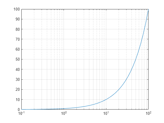
Create a vector of logarithmically spaced x-coordinates and two vectors of y-coordinates. Plot two lines by passing comma-separated x-y pairs to semilogx.
x = logspace(-1,2);
y1 = x;
y2 = -x;
semilogx(x,y1,x,y2)
grid on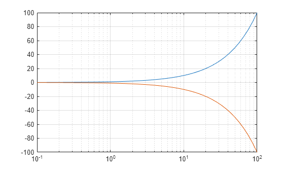
Define f as a vector containing the frequencies from 10 Hz to 100,000 Hz. Define gain as a vector of power gain values in decibels. Then plot the gain values against frequency.
f = logspace(1,5,100);
v = linspace(-50,50,100);
gain = (1-exp(5*(2.5*v.^2)./7500))/14;
semilogx(f,gain)
grid on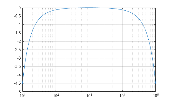
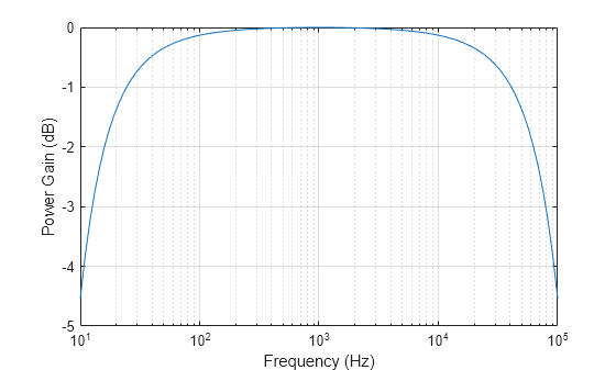
Call the yticks function to reposition the y-axis tick values at whole-number increments along the y-axis. Then create x- and y-axis labels by calling the xlabel and ylabel functions.
yticks([-5 -4 -3 -2 -1 0])
xlabel ('Frequency (Hz)')
ylabel('Power Gain (dB)')
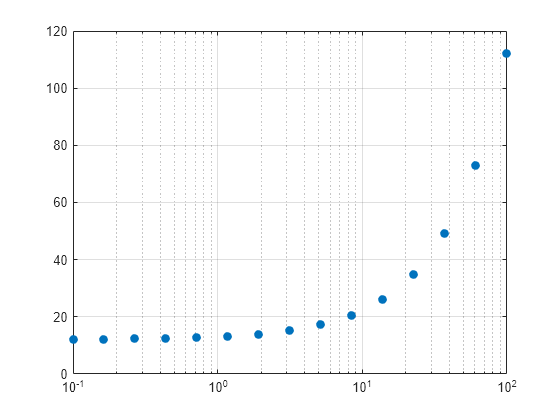
Create a set of x- and y-coordinates and display them in a linear-log plot. Specify the line style as 'o' to display circular markers without connecting lines. Specify the marker fill color as the RGB triplet [0 0.447 0.741], which corresponds to a dark shade of blue.
x = logspace(-1,2,15);
y = 12 + x;
semilogx(x,y,'o','MarkerFaceColor',[0 0.447 0.741])
grid on
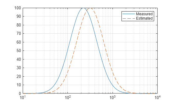
Create a vector of logarithmically spaced x-coordinates and two vectors of y-coordinates. Then plot two lines by passing comma-separated x-y pairs to semilogx. Display a legend by calling the legend function.
x = logspace(1,4,100);
v = linspace(-50,50,100);
y1 = 100*exp(-1*((v+5).^2)./200);
y2 = 100*exp(-1*(v.^2)./200);
semilogx(x,y1,x,y2,'--')
legend('Measured','Estimated')
grid on
When you specify only one coordinate vector, semilogx plots those coordinates against the values 1:length(y). For example, define y as a vector of 5 values between 0 and 40. Create a linear-log plot of y.
y = [0 10 20 30 40];
semilogx(y)
grid on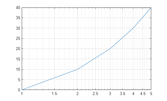
If you specify y as a matrix, the columns of y are plotted against the values 1:size(y,1). For example, define y as a 5-by-3 matrix and pass it to the semilogx function. The resulting plot contains 3 lines, each of which has x-coordinates that range from 1 to 5.
y = [ 0    10    20
     10    20    30
     20    30    40
     30    40    50
     40    50    60];

semilogx(y)
grid on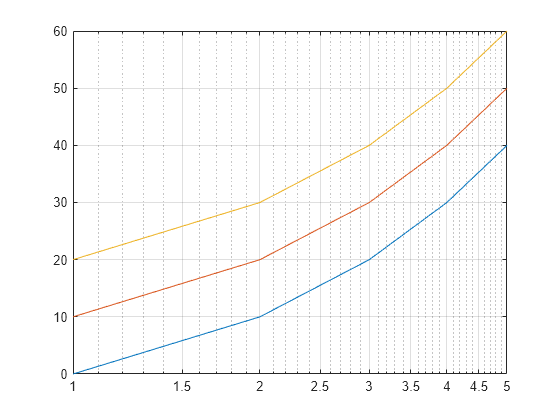
Since R2022a
A convenient way to plot data from a table is to pass the table to the semilogx function and specify the variables to plot.
Create a table containing two variables. Then display the first three rows of the table.
Input = logspace(-1,2)';
Output = 2*Input;
tbl = table(Input,Output);
head(tbl,3)
     Input     Output
    _______    _______

        0.1        0.2
    0.11514    0.23028
    0.13257    0.26514
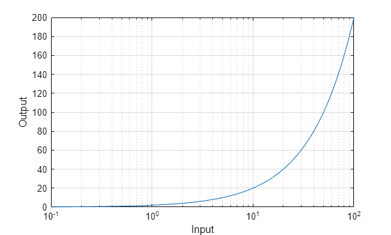
Plot the Input variable on the x-axis and the Output variable on the y-axis. Return the Line object as p, and turn the axes grid on. Notice that the axis labels match the variable names.
p = semilogx(tbl,"Input","Output");
grid on
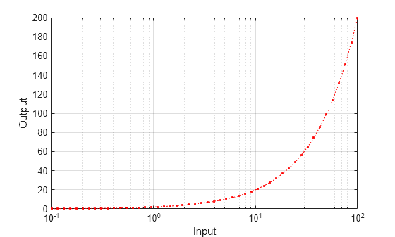
To modify aspects of the line, set the LineStyle, Color, and Marker properties on the Line object. For example, change the line to a red dotted line with point markers.
p.LineStyle = ":";
p.Color = "red";
p.Marker = ".";
Since R2022a
Create a table containing three variables. Then display the first three rows in the table.
Input = logspace(-1,2)';
Output1 = 2*Input;
Output2 = -Input;
tbl = table(Input,Output1,Output2);
head(tbl,3)
     Input     Output1    Output2
    _______    _______    ________

        0.1        0.2        -0.1
    0.11514    0.23028    -0.11514
    0.13257    0.26514    -0.13257
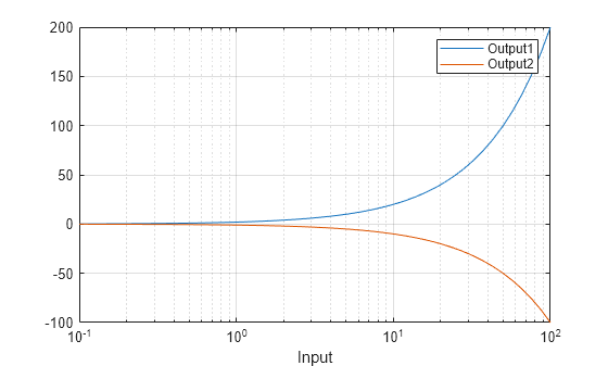
Plot the Input variable on the x-axis and the Output1 and Output2 variables on the y-axis. Add a legend. Notice that the legend labels match the variable names.
semilogx(tbl,"Input",["Output1" "Output2"])
grid on
legend
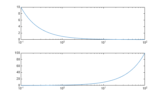
Create a tiled chart layout in the 'flow' tile arrangement, so that the axes fill the available space in the layout. Next, call the nexttile function to create an axes object and return it as ax1. Then display a linear-log plot by passing ax1 to the semilogx function.
tiledlayout('flow')
ax1 = nexttile;
x = logspace(-1,2);
y1 = 1./x;
semilogx(ax1,x,y1)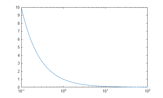
Repeat the process to create a second linear-log plot.
ax2 = nexttile;
y2 = x;
semilogx(ax2,x,y2)
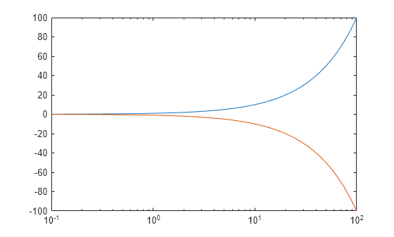
Create a linear-log plot containing two lines, and return the line objects in the variable slg.
x = logspace(-1,2);
y1 = x;
y2 = -x;
slg = semilogx(x,y1,x,y2);
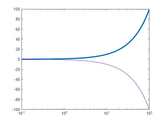
Change the width of the first line to 3, and change the color of the second line to purple.
slg(1).LineWidth = 3;
slg(2).Color = [0.4 0 1];
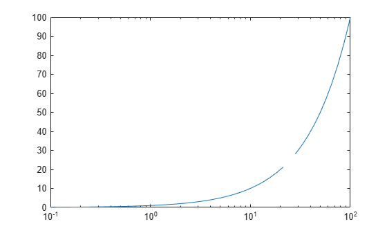
Insert NaN values wherever there are discontinuities in your data. The semilogx function displays gaps at those locations.
Create a pair of x- and y-coordinate vectors. Replace the fortieth y-coordinate with a NaN value. Then create a linear-log plot of x and y.
x = logspace(-1,2);
y = x;
y(40) = NaN;
semilogx(x,y)
Input Arguments
Log scale coordinates, specified as a scalar, vector, or matrix. The size and shape
of X depends on the shape of your data and the type of plot you want
to create. This table describes the most common situations.
| Type of Plot | How to Specify Coordinates |
|---|---|
| Single point | Specify semilogx(1,2,'o') |
| One set of points | Specify semilogx([1 2 3],[4; 5; 6]) |
| Multiple sets of points (using vectors) | Specify consecutive pairs of semilogx([1 2 3],[4 5 6],[1 2 3],[7 8 9]) |
| Multiple sets of points (using matrices) | If all the sets share the same x- or y-coordinates, specify the shared coordinates as a vector and the other coordinates as a matrix. The length of the vector must match one of the dimensions of the matrix. For example: semilogx([1 2 3],[4 5 6; 7 8 9]) semilogx plots one line for each
column in the matrix. Alternatively, specify
semilogx([1 2 3; 4 5 6],[7 8 9; 10 11 12]) |
semilogx might exclude coordinates in some cases:
If the log scale coordinates include positive and negative values, only the positive values are displayed.
If the log scale coordinates are all negative, all of the values are displayed on a log scale with the appropriate sign.
Log scale values of zero are not displayed.
Data Types: single | double | int8 | int16 | int32 | int64 | uint8 | uint16 | uint32 | uint64
Linear scale coordinates, specified as a scalar, vector, or matrix. The size and
shape of Y depends on the shape of your data and the type of plot you
want to create. This table describes the most common situations.
| Type of Plot | How to Specify Coordinates |
|---|---|
| Single point | Specify semilogx(1,2,'o') |
| One set of points | Specify semilogx([1 2 3],[4; 5; 6]) |
| Multiple sets of points (using vectors) | Specify consecutive pairs of semilogx([1 2 3],[4 5 6],[1 2 3],[7 8 9]) |
| Multiple sets of points (using matrices) | If all the sets share the same x- or y-coordinates, specify the shared coordinates as a vector and the other coordinates as a matrix. The length of the vector must match one of the dimensions of the matrix. For example: semilogx([1 2 3],[4 5 6; 7 8 9]) semilogx plots one line for each
column in the matrix.Alternatively, specify
semilogx([1 2 3; 4 5 6],[7 8 9; 10 11 12]) |
Data Types: single | double | int8 | int16 | int32 | int64 | uint8 | uint16 | uint32 | uint64 | categorical | datetime | duration
Line style, marker, and color, specified as a string scalar or character vector containing symbols. The symbols can appear in any order. You do not need to specify all three characteristics (line style, marker, and color). For example, if you omit the line style and specify the marker, then the plot shows only the marker and no line.
Example: "--or" is a red dashed line with circle markers.
| Line Style | Description | Resulting Line |
|---|---|---|
"-" | Solid line |
|
"--" | Dashed line |
|
":" | Dotted line |
|
"-." | Dash-dotted line |
|
| Marker | Description | Resulting Marker |
|---|---|---|
"o" | Circle |
|
"+" | Plus sign |
|
"*" | Asterisk |
|
"." | Point |
|
"x" | Cross |
|
"_" | Horizontal line |
|
"|" | Vertical line |
|
"square" | Square |
|
"diamond" | Diamond |
|
"^" | Upward-pointing triangle |
|
"v" | Downward-pointing triangle |
|
">" | Right-pointing triangle |
|
"<" | Left-pointing triangle |
|
"pentagram" | Pentagram |
|
"hexagram" | Hexagram |
|
| Color Name | Short Name | RGB Triplet | Appearance |
|---|---|---|---|
"red" | "r" | [1 0 0] |
|
"green" | "g" | [0 1 0] |
|
"blue" | "b" | [0 0 1] |
|
"cyan"
| "c" | [0 1 1] |
|
"magenta" | "m" | [1 0 1] |
|
"yellow" | "y" | [1 1 0] |
|
"black" | "k" | [0 0 0] |
|
"white" | "w" | [1 1 1] |
|
Source table containing the data to plot, specified as a table or timetable.
Table variables containing the x-coordinates, specified using one of the indexing schemes from the table.
| Indexing Scheme | Examples |
|---|---|
Variable names:
|
|
Variable indices:
|
|
Variable type:
|
|
The table variables you specify can contain any numeric values. However,
semilogx might exclude negative and zero values from the plot in
the same way as it does when you specify X as a vector containing
negative or zero values.
If xvar and yvar both specify multiple
variables, the number of variables must be the same.
Example: semilogx(tbl,["x1","x2"],"y") specifies the table
variables named x1 and x2 for the
x-coordinates.
Example: semilogx(tbl,2,"y") specifies the second variable for the
x-coordinates.
Example: semilogx(tbl,vartype("numeric"),"y") specifies all
numeric variables for the x-coordinates.
Table variables containing the y-coordinates, specified using one of the indexing schemes from the table.
| Indexing Scheme | Examples |
|---|---|
Variable names:
|
|
Variable indices:
|
|
Variable type:
|
|
The table variables you specify can contain numeric, categorical, datetime, or
duration values. If xvar and yvar both specify
multiple variables, the number of variables must be the same.
Example: semilogx(tbl,"x",["y1","y2"]) specifies the table
variables named y1 and y2 for the
y-coordinates.
Example: semilogx(tbl,"x",2) specifies the second variable for the
y-coordinates.
Example: semilogx(tbl,"x",vartype("numeric")) specifies all
numeric variables for the y-coordinates.
Target axes, specified as an Axes object. If you do not specify
the axes and if the current axes is Cartesian, then semilogx uses the
current axes.
Name-Value Arguments
Specify optional pairs of arguments as
Name1=Value1,...,NameN=ValueN, where Name is
the argument name and Value is the corresponding value.
Name-value arguments must appear after other arguments, but the order of the
pairs does not matter.
Before R2021a, use commas to separate each name and value, and enclose
Name in quotes.
Example: semilogx([1 2],[3 4],'Color','red') specifies a red line for
the plot.
Note
The properties listed here are only a subset. For a complete list, see Line Properties.
Color, specified as an RGB triplet, a hexadecimal color code, a color name, or a
short name. The color you specify sets the line color. It also sets the marker edge
color when the MarkerEdgeColor property is set to
'auto'.
For a custom color, specify an RGB triplet or a hexadecimal color code.
An RGB triplet is a three-element row vector whose elements specify the intensities of the red, green, and blue components of the color. The intensities must be in the range
[0,1], for example,[0.4 0.6 0.7].A hexadecimal color code is a string scalar or character vector that starts with a hash symbol (
#) followed by three or six hexadecimal digits, which can range from0toF. The values are not case sensitive. Therefore, the color codes"#FF8800","#ff8800","#F80", and"#f80"are equivalent.
Alternatively, you can specify some common colors by name. This table lists the named color options, the equivalent RGB triplets, and the hexadecimal color codes.
| Color Name | Short Name | RGB Triplet | Hexadecimal Color Code | Appearance |
|---|---|---|---|---|
"red" | "r" | [1 0 0] | "#FF0000" |
|
"green" | "g" | [0 1 0] | "#00FF00" |
|
"blue" | "b" | [0 0 1] | "#0000FF" |
|
"cyan"
| "c" | [0 1 1] | "#00FFFF" |
|
"magenta" | "m" | [1 0 1] | "#FF00FF" |
|
"yellow" | "y" | [1 1 0] | "#FFFF00" |
|
"black" | "k" | [0 0 0] | "#000000" |
|
"white" | "w" | [1 1 1] | "#FFFFFF" |
|
"none" | Not applicable | Not applicable | Not applicable | No color |
This table lists the default color palettes for plots in the light and dark themes.
| Palette | Palette Colors |
|---|---|
Before R2025a: Most plots use these colors by default. |
|
|
|
You can get the RGB triplets and hexadecimal color codes for these palettes using the orderedcolors and rgb2hex functions. For example, get the RGB triplets for the "gem" palette and convert them to hexadecimal color codes.
RGB = orderedcolors("gem");
H = rgb2hex(RGB);
Before R2023b: Get the RGB triplets using RGB =
get(groot,"FactoryAxesColorOrder").
Before R2024a: Get the hexadecimal color codes using H =
compose("#%02X%02X%02X",round(RGB*255)).
Tips
The
semilogxfunction uses colors and line styles based on theColorOrderandLineStyleOrderproperties of the axes.semilogxcycles through the colors with the first line style. Then, it cycles through the colors again with each additional line style.You can change the colors and the line styles after plotting by setting the
ColorOrderorLineStyleOrderproperties on the axes. You can also call thecolororderfunction to change the color order for all the axes in the figure.
Algorithms
The semilogx function plots x-coordinates on a log
scale by setting the XScale property of the axes to
'log'. However, if the axes hold state is 'on' before you call
semilogx, the property does not change, and the
x-coordinates might display on a linear scale.
Extended Capabilities
Version History
Introduced before R2006aWhen you pass a table and one or more variable names to the semilogx function, the axis and legend labels now display any special characters that are included in the table variable names, such as underscores. Previously, special characters were interpreted as TeX or LaTeX characters.
For example, if you pass a table containing a variable named Sample_Number
to the semilogx function, the underscore appears in the axis and
legend labels. In R2022a and earlier releases, the underscores are interpreted as
subscripts.
| Release | Label for Table Variable "Sample_Number" |
|---|---|
R2022b |
|
R2022a |
|
To display axis and legend labels with TeX or LaTeX formatting, specify the labels manually.
For example, after plotting, call the xlabel or
legend function with the desired label strings.
xlabel("Sample_Number")
legend(["Sample_Number" "Another_Legend_Label"])