Assess Local Models

R2026b

How to Assess Local Models

After fitting models using a two-stage test plan in the Model Browser, you must assess local models, then global models, and then create the two-stage model. When you select a local node (with the icon) in the Model Browser tree, the local level view appears. At the local level you can:

View local model plots and statistics, and scroll through all local models operating point by operating point. See Using Local Model Plots, and Viewing Local Model Statistics.
Look for problem operating points with the RMSE Plots. See Using the RMSE Plot with Local Models.
You can use the Operating Point Notes pane to record information on particular operating points.
Remove and restore outliers and update fits. See Removing Outliers and Updating Fits.
Calculate two-stage models, and add or remove response features. After calculating the two-stage model, you can compare the local fit and the two-stage fit on the local level plots. See Create Two-Stage Models.

Note that after the two-stage model is calculated the local node icon changes to a two-stage icon ( ) to reflect this. The response node also has a two-stage icon, but produces the response level view instead.

Using Local Model Plots

Sweep Plot

You can scroll through all the local models by using the up and down operating point buttons, type directly in the edit box, or go directly to operating point numbers by clicking Select Operating Point.

The sweep plot shows the local model fit to the data for the current operating point only, with the datum point if there is a datum model. If there are multiple inputs to the local model, a predicted/observed plot is displayed. In this case to examine the model surface in more detail you can use Model > Evaluate. See Model Evaluation Window.

To examine the local fit in more detail, close other plots, or zoom in on parts of the plot by Shift-click-dragging or middle-click-dragging on the place of interest on the plot. Return to full size by double-clicking.

Diagnostic Statistics Plot

The Diagnostic Statistics plot can show various scatter plots of statistics for assessing goodness-of-fit for the current local model shown. The statistics available for plotting are model dependent.

Dropdown menu with options: spark (L1) [deg], Residuals, Weighted residuals, Studentized residuals (highlighted), tq [ft lbf], Predicted tq [ft lbf], Leverage, and Obs. number.

The preceding is an example drop-down menu on the scatter plot for changing x and y factors. In this case spark is the local input factor and torque is the response. The local inputs, the response, and the predicted response are always available in these menus. The observation number is also always available.

The other options are statistics that are model dependent, and can include residuals, weighted residuals, studentized residuals, and leverage. At local level these are internally studentized residuals.

Using the RMSE Plot with Local Models

Use the RMSE Plot to quickly identify problem operating points and navigate to an operating point of interest. The plot shows the standard errors of all the operating points, both overall and by response feature. Navigate to an operating point of interest by double-clicking a point in the plot to select the operating point in the other plots in the local model view.

The plot displays one value of standard error per operating point, overall and for each response feature. As a best practice, first plot RMSE against operating point number to get an idea of how the error is distributed and locate any operating points with much higher errors. Right-click to toggle display of operating point numbers. Ideally, all the standard errors should be roughly the same value to satisfy the statistical assumptions for two-stage models. If these assumptions are not satisfied, error estimates for two-stage models may not be valid.

You can also use the X- and Y-axis factor drop-down lists to plot these standard errors against the global variables to examine the global distribution of error.

Additional Plots

You can add or change plots by clicking the toolbar buttons, split buttons in plot title bars, or selecting an option from Current View in the context menu or View menu. You can add:

Data Plots — View plots of the data for the current operating point. Select View > Plot Variables to choose variables to plot. You can choose to view any of the data signals in the data set for the current operating point (including signals not being used in modeling). You can plot a pair of variables or plot a variable against record number. You can add more data plots if you want.
Note
You can also view values of global variables in the Global variables pane.
Normal Plot — Normal plots are a useful graph for assessing whether data comes from a normal distribution. For more information, see Normal Probability Plots.
Validation Data If you are using validation data, the plot shows the local model validation residuals if there is validation data for the current operating point (the global variables must match). If there is a two-stage model, the two-stage validation residuals are also shown. Validation data must be attached at the Edit Test Plan Definition. See Using Validation Data.
Model Definition — View the parameters and coefficients of the model formula and the scaling details.

Removing and Restoring Outliers

You can use the right-click context menus on plots or the Outliers menu to remove and restore outliers. For available options, see Remove and Restore Outliers.

Local models have an additional option to remove a whole operating point: Outliers > Remove All Data. This option leaves the current local model with no data, so entirely removes the current operating point. This operating point is removed from all the global models.

Updating Other Fits

When you remove an outlier from your local model, it refits immediately. Other dependent fits also need updates. You can choose when to update the other fits. Removing an outlier can affect several other models. Removing an outlier from a best local model changes all the response features for that two-stage model. The global models all change; therefore the two-stage model must be recalculated. For this reason the local model node returns to the local (house) icon and the response node becomes blank again. If the two-stage model has a datum model defined, and other models within the test plan are using a datum link model, they are similarly affected.

To update fits, either:

In the local view, use the Update Fit toolbar button to update all the dependent fits.
When you select another model node, you are prompted to update or defer updates.
When leaving the local node, a dialog box asks if you want to update all dependent fits. Click Yes to update all global models, or No to delay lengthy updates of dependent fits. Delaying updates can be useful when you want to examine only a particular global model after removing an outlier at the local level. With the defer option, you can avoid waiting while updating all other dependent fits.
If you defer updating fits and you go to a response feature node, the toolbox refits only that node, so you can inspect that global model fit. Other response features do not update unless you click them. When you return to the local node again the Update Fit button is enabled. Until you update fits, a status message at the bottom of the browser tells you that you have deferred updates.

Create Two-Stage Models

To create a two-stage model, click Create Two-Stage in the Common Tasks pane.

If your model supports it, you are prompted to calculate the two-stage model using maximum likelihood estimation (MLE). This takes correlations between response features into account.

Note

You need the right number of response features to create a two-stage model. You are prompted if you need to select response features, then the toolbox creates the two-stage model.

After creating the two-stage model, compare the local fit and the two-stage fit on the local level plots.

MLE Settings

Calculating MLE: For an ordinary (univariate) two-stage model, the global models are created in isolation without accounting for any correlations between the response features.

Using MLE (maximum likelihood estimation) to fit the two-stage model takes account of possible correlations between response features.
In cases where such correlations occur, using MLE significantly improves the two-stage model.

When you click Create Two-Stage Model in the common tasks pane, and your model support MLE, then a dialog box asks if you want to calculate MLE. If you click Cancel at this point, you can calculate MLE later as follows:

From the local node, click the MLE icon in the toolbar .
Alternatively, choose Model > Calculate MLE.
The MLE dialog box appears. Click Start.
After you click Start a series of progress messages appears, then a new Two-Stage RMSE (root mean squared error) value is reported.
You can perform more iterations by clicking Start again to see how the RMSE value changes, or you can click Stop at any time.
Clicking OK returns you to the Model Browser, where you can view the new MLE model fit.
After calculating MLE, notice that the plots and the icons in the model tree for the whole two-stage model (response node, local node, and all response feature nodes) have turned purple.

You can select all response features in turn to inspect their properties graphically; the plots are all purple to symbolize MLE. At the local node the plots show the purple MLE curves against the black local fit and the blue data.

From the response feature nodes, at any time, click the MLE toolbar icon to recalculate MLE and perform more iterations.
From the local node, you can open the Model Selection window to compare the MLE model with the previous univariate model (without correlations), and choose the best. Here you can select the univariate model and click Assign Best to “undo” MLE and return to the previous model.

MLE dialog box settings:

Algorithm
The algorithm drop-down menu offers a choice between two covariance estimation algorithms, Quasi-Newton and Expectation Maximization. These are algorithms for estimating the covariance matrix for the global models.
Quasi-Newton is recommended for smaller problems (< 5 response features and < 100 operating points). Quasi-Newton usually produces better answers (smaller values of -logL) and hence is the default for small problems.
Expectation Maximization is an iterative method for calculating the global covariance (as described in Davidian and Giltinan (1995); see References in Two-Stage Models for Engines). This algorithm has slow convergence, so you might want to use the Stop button.
Tolerance
You can edit the tolerance value. Tolerance is used to specify a stopping condition for the algorithm. The default values are usually appropriate, and if calculation is taking too long you can always click Stop.
Initialize with previous estimate
When you recalculate MLE (that is, perform more iterations), there is a check box you can use to initialize with the previous estimate.
Predict missing values
The other check box (selected by default) predicts missing values. When it is selected, response features that are outliers for the univariate global model are replaced by the predicted value. This allows operating points to be used for MLE even if one of the response features is missing. If all the response features for a particular operating point are missing or the check box is unselected, the whole operating point is removed from MLE calculation.

Create Alternative Local and Global Models

To quickly build a selection of alternative global models to compare, in the Common Tasks pane, click Build Global Models. This opens the Model Template dialog box. For local models, you build a selection of child nodes for each response feature node. See Create Alternative Models to Compare for details.
The toolbox selects the best model for each response feature, based on your selection criteria (such as AICc). Assess all the fits in case you want to choose an alternative.
To change the current local model type, in the Common Tasks pane, click Edit Model. This opens the Model Setup dialog box, where you can choose another model type. See Explore Local Model Types.
Model > Fit Local — Opens the Local Model Fit Tool dialog box. If you are covariance modeling, you can choose three algorithms: REML (Restricted Maximum Likelihood - the default), Pseudo-likelihood, or Absolute residuals. Using the Fit button might take several steps to converge, but if you use the One Step button only one step in the optimization process is taken. Every time you run a process, the initial and final Generalized Least Squares parameter values are displayed for each iteration.
Without covariance modeling, you can only click Fit. The Ordinary Least Squares (OLS) parameters are displayed. Click Fit to rerun. You can enter a different change in parameters in the edit box.

After creating alternative models, for next steps, see Compare Alternative Models.

Viewing Local Model Statistics

Local Statistics Pane
Pooled Statistics

Local Statistics Pane

You can select the information to display in the Local Statistics pane.

Summary statistics — RMSE for the current operating point, number of observations, degrees of freedom on the error, R squared, Cond(J) (the condition index for the Jacobian matrix).

Note
Check for high values of Cond(J) (e.g., > 10⁸). High values of this condition indicator can be a sign of numerical instability.

If there is validation data for the current operating point, Validation RMSE for the current operating point also appears here.
Parameters — Shows the values and standard errors of the parameters in the local model for the current operating point selected.
Correlations — Shows a table of the correlations between the parameters.
Response Features — Shows the values and standard errors of the response features defined for this local model, from the current operating point (often some or all of them are the same as the parameters; others are derived from the parameters).
Global Covariance — For MLE models, shows a covariance matrix for the response features at the global level.

The Global variables pane shows the values and standard errors of the global variables at the position of the current operating point.

Pooled Statistics

These are seen at the local node (when two-stage modeling) in the Pooled Statistics table, and at the response node in the list of local models. If you have a selection of local or two-stage models, use these statistics to help you choose which model is best.

Local RMSE	Root mean squared error between the local model and the data for all operating points. The divisor used for RMSE is the number of observations minus the number of parameters.
Two-Stage RMSE	Root mean squared error between the two-stage model and the data for all operating points. You want this error to be small for a good model fit.
PRESS RMSE	Root mean squared error of predicted errors, useful for indicating overfitting; see PRESS statistic. The divisor used for PRESS RMSE is the number of observations. Not displayed for MLE models because the simple univariate formula cannot be used.
Two-Stage T^2	T^2 is a normalized sum of squared errors for all the response features models. You can see the basic formula on the Likelihood view of the Model Selection window. Where , where C_iis the local covariance for operating point i. See blockdiag diagram following. A large T^2 value indicates that there is a problem with the response feature models.
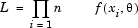
-log L	Log-likelihood function: the probability of a set of observations given the value of some parameters. You want the likelihood to be large, tending toward -infinity, so large negative is good. For n observations x₁,x₂,..x_n, with probability distribution , the likelihood is: This is the basis of MLE. See Create Two-Stage Models. which is the same as: This assumes a normal distribution. You can view plots of -log L in the Model Selection window, see Likelihood View.
Validation RMSE	Root mean squared error between the two-stage model and the validation data for all operating points.

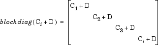
To explain blockdiag as it appears under T^2 in the Pooled statistics table: , where C_iis the local covariance for operating point i, is calculated as shown below.