Define Design Constraints

R2026b

In many cases, designs might not coincide with the operating region of the system to be tested. For example, an automobile engine normally does not operate in a region of low speed (n) and high exhaust gas recirculation (EGR). You cannot run 15% EGR at 1000 RPM. Selecting design points in impractical regions serves no purpose, so you can constrain the candidate set for test point generation.

Designs can be constrained by geometric relationships or by boundaries defined by the operating limits of the system under test. This table shows the different constraint types and provides guidance on when to use each, along with example use cases.

Constraint Type	Use Case	Example	More Info
1D Table	You want to restrict a single variable to a valid interval or value.	Limiting spark advance to avoid knock Limiting air-fuel enrichment to protect catalyst Limiting turbo speed to stay below the surge speed limit	1D Table Constraints
2D Table	You need to restrict two variables together, defining a region in a plane.	Turbocharger mass flow vs pressure ratio map to prevent operating left of the surge line Fuel injection timing vs fuel rail pressure to avoid cavitation or excessive soot formation regions	2D Table Constraints
Linear	You want flat constraints for fast computation.	Satisfying a feasible torque request based on spark and air inputs Constraining based on fuel economy vs emissions tradeoff	Linear Constraints
Ellipsoid	You need to represent an uncertainty or feasible region with a curved boundary.	Modeling misfire or stability limits as ellipsoids representing air-fuel ratio, spark, and EGR	Ellipsoid Constraints
Boundary	You want to constrain the space based on the operating limits of the system.	Limiting testing to maximum torque output of hardware	Explore Boundary Model Types

Add and View Constraints

Note

When you add constraints, the design type changes to Custom (except optimal designs). For space-filling and classical designs, you can no longer access the original design generation settings in the Design Properties dialog box. If you want to preserve your original design settings, create a child design to constrain. This step is important if you want to augment a space-filling design. See Augmenting Space-Filling Designs.

To add a constraint to a design:

1. In the Design Editor, select Edit > Constraints.

2. In the Constraints Manager dialog box, you can add new constraints, and you can delete, edit, duplicate or negate existing constraints. Use the NOT button to negate a constraint, for example, if you want to constrain points to be outside a boundary model.

If there are no constraints yet, the Constraints Manager is empty, and you can only click Add to construct a new constraint.

To construct a new constraint:

1. Click Add.

2. The Edit Constraint dialog box opens. You can set the Constraint type to: Linear, Ellipsoid, 1D Table, or 2D table. See Constraint Types.

3. After defining any constraint, click OK. Your new constraint appears in the Constraints Manager. Click OK to return to the Design Editor, or click Add to define more constraints.

A dialog box appears if points in the design fall outside your newly constrained candidate set. You can continue (delete them) or cancel the constraint. Fixed points are not removed by this process. For optimal designs, you can also replace them with new random points within the new candidate set, as shown in the preceding example figure.

Note

The Replace option is only available for optimal designs. If you want to replace points removed by constraints from other designs, you can select Edit > Add Point to add points optimally, randomly, or at chosen places. However, if so many points have been removed by a constraint that not enough remain left to fit the current model, optimal addition is not possible. See Adding and Editing Design Points.

To view constraints in the Design Editor:

1. Right-click the Design Editor display pane to reach the context menu.

2. Select Current > View > 3D Constraints. (You can also select 2D constraints view.)

   

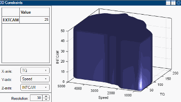
Use these views to better understand the region of space that is currently available within the constraint boundaries.

Constraint Types

Available constraint types include 1D table, 2D table, linear, and ellipsoid. These constraint types are the same in the Design Editor and in optimizations in the CAGE Browser.

1D Table Constraints

1D table constraints limit the maximum or minimum setting of one factor as a function of another factor. Linear interpolation between user-defined points is used to specify the constraint. You can use either the edit boxes or the plot to define the constraint.

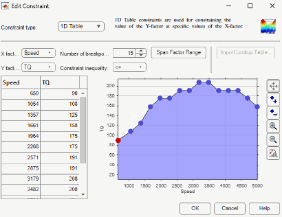
• Select the appropriate factors to use for X and Y, and choose whether to constrain above or below the defined boundary using the Constraint inequality list.

• You can enter a value for Number of breakpoints, click the Span Factor Range button to space your breakpoints evenly, and enter breakpoint values into the table. You can use a CAGE table or normalizer to define a constraint. If CAGE is open and contains a suitable table, you can click Import Lookup Table.

• On the plot, you can add and remove points using the buttons and click and drag the points to define the boundary. You can also enter values in the edit boxes for the selected point.

Linear Constraints

You specify the coefficients of the equation for an N-1 dimensional hyperplane in the N-factor space. The form of the equation is $$A.x=b$$, where A is your defined coefficient vector, x is the vector of values of the factors, to be constrained, and b is a scalar. For example, in two dimensions: $$\text{A=(1,2)}$$, $$x=(L,A)$$, $$b=3$$.

Then, $$A.x=b$$ expands to $$1\times L+2\times A=3$$.

You can rearrange this equation and write it as $$A=-\frac{L}{2}+\frac{3}{2}$$, which corresponds to the traditional equation of a 2D straight line, $$y=mx+c$$, with $$m=-\frac{1}{2}$$ and $$c=\frac{3}{2}$$.

$$A.x=b$$ is thus the higher dimensional extension of this equation.

The linear constraints work by selecting the region below the defined plane (that is, $$A.x\le b$$). To select a region above the plane, multiply all your values by -1: A becomes -A, b becomes -b.

For example, to select a simple plane where SPK<50 as a constraint boundary, enter 1 next to SPK and 50 next to b. You can set all the other factors to 0, or you can remove them on the Inputs tab if you are constraining an optimization.

Ellipsoid Constraints

The ellipsoid constraint allows you to define an N-dimensional ellipsoid. You can specify the center of the ellipsoid, the length of each axis, and the rotation of the ellipsoid.

Ellipsoid center.  You can specify the center of the ellipsoid by entering values in the Center point columns. These values, in natural units, mark where you want the ellipsoid to be centered in each of the factor dimensions. The defaults are the midpoint of each factor range.

Axis length.  You specify the size of the ellipsoid by entering values along the diagonal of the matrix. The default values create an ellipsoid that touches the edge of the space in each of the factor dimensions. In general, for an entry value X in the diagonal, the ellipsoid size in that factor is $$\frac{1}{\sqrt{x}}$$.

If you want a radius of r in a factor, enter 1/(r^2). For example, if you want to restrict N to a radius of 2000 from the center point, enter 1/2000^2 = 2.5e-7.

Enter a zero in the diagonal to not constrain with respect to that factor.

Rotation.  The matrix entries that are not on the main diagonal control rotation of the ellipsoid.

This example shows a defined ellipsoid constraint.

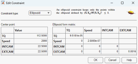
You must enter values in the table to define the ellipsoid. If you leave the values at the defaults, the candidate set is an ellipsoid that spans the factor ranges.

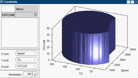
In this example, entering 2.5e-7 in the ENGSPEED diagonal restricts that axis to 1/sqrt(2.5e-7) = 2000. Entering zero in the INTCAM diagonal leaves INTCAM unconstrained (that is, the constraint is a cylinder extending to the ends of the INTCAM factor range). The ellipsoid is not rotated as the nondiagonal matrix entries are all zero.

This 3D display shows the shape of this example constraint in the Design Editor.

2D Table Constraints

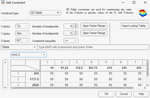
2D table constraints are an extension of the 1D table. Constraint boundary values for a factor are specified over a 2D grid of two other factors.

• You can specify these grid locations by entering values in the top row and left column, while the matrix of values for the third factor is entered in the rest of the edit boxes. To specify grid values, you can enter values directly or choose the number of breakpoints for your grid and space them over the factors' ranges, using the controls described below.

• You can specify the number of breakpoints for the X and Y factors.

• To space your breakpoints evenly over the range of X or Y, click Span Range. This step is useful if you add some breakpoints, as new points are often all at the maximum value for that factor. Using the Span Range button is faster than changing points manually.

• You can specify to keep the region below (<=) or above (>=) the constraint boundary, as for the 1D table, using the Constraint inequality drop-down list for the Z factor.

• You can switch to coded values using the check box.

The constraint boundary between the defined grid points is calculated using bilinear interpolation.

Importing Constraints

Select Edit > Constraints. In the Constraints Manager dialog box, click Import.

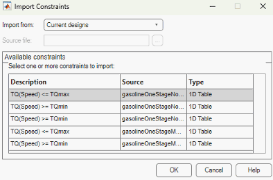
In the Import Constraints dialog box, select where you want to import the constraints from.

Import Source	Description
Current designs	Import any existing constraints in the design tree.
Design Editor file (*.mvd)	Extract constraints from a design file.
Boundary Constraints (current project)	Import boundary constraints from the Model Browser project.
Boundary Constraints (*.mat file)	Extract boundary constraints from a file.
Classifiers	Import classifiers from the workspace. Use classifiers to differentiate between good and bad operating conditions when you specify boundary constraints for design experiments. To create support vector machines (SVMs) or discriminant classifiers: Use the Statistics and Machine Learning Toolbox™ to classify data. Use the Classification Learner App to export the classification model to the workspace.

Note

You can only import design constraints from designs that have the same number of factors and have the same coded range for each factor. For designs of N factors, you can import boundary constraints with N or fewer active factors.

1. If importing from a file, you can type the filename in the edit box or use the browse button to locate the file.

2. Click to select constraints in the Available Constraints list, or Ctrl+click to select multiple constraints.

3. Click OK to import and apply the constraints.

   If importing boundary constraints, a dialog box appears for each constraint where you can match up factor names.