phased.IntensityScope
Range-time-intensity (RTI) or Doppler-time-intensity (DTI) display
Description
The phased.IntensityScope
System object™ creates an intensity scope for viewing range-time-intensity (RTI) or
Doppler-time-intensity (DTI) data. An intensity scope is a scrolling waterfall of intensity
values as a function of time. Scan lines appear at the bottom of the display window and scroll
off at the top. Each scan line represents signal intensity as a function of a parameter of
interest, such as range or speed. You can also use this object to display angle-time-intensity
data and spectral data. This figure shows an RTI display.
To create an intensity scope:
Create the
phased.IntensityScopeobject and set its properties.Call the object with arguments, as if it were a function.
To learn more about how System objects work, see What Are System Objects?
Creation
Description
sIS = phased.IntensityScopesIS, having default property values.
sIS = phased.IntensityScope(Name=Value)sIS, with each specified property
Name set to a specified Value. You can specify
several name-value arguments in any order as
Name1=Value1,...,NameN=ValueN.
Properties
Usage
Syntax
Description
sIS(data)data.
Note
The object performs an initialization the first time the object is executed. This
initialization locks nontunable properties
and input specifications, such as dimensions, complexity, and data type of the input data.
If you change a nontunable property or an input specification, the System object issues an error. To change nontunable properties or inputs, you must first
call the release method to unlock the object.
Input Arguments
Object Functions
To use an object function, specify the
System object as the first input argument. For
example, to release system resources of a System object named obj, use
this syntax:
release(obj)
Examples
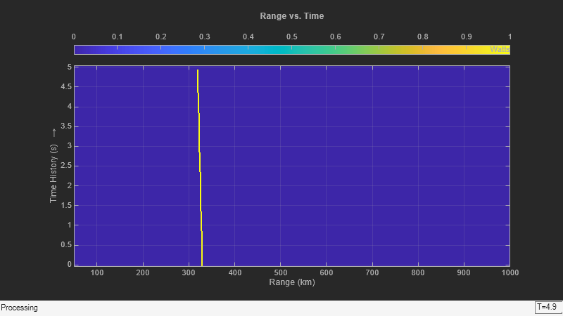
Use a phased.IntensityScope System object™ to display the echo intensity of a moving target as a function of range and time.
Run the simulation for 5 seconds at 0.1 second steps. In the display, each horizontal scan line shows the intensities of radar echo at each time step.
nsteps = 50;
dt = .1;
timespan = nsteps*dt;
Simulate a target at a range of 320.0 km and a range rate of 2.0 km/s. Echoes are resolved into range bins of 1 km resolution. The range bins span from 50 to 1000 km.
rngres = 1.0;
rngmin = 50.0;
rngmax = 1000.0;
tgtrange = 320.0;
rangerate = 2.0;
rngscan = [rngmin:rngres:rngmax];
Set up the Intensity Scope using these properties.
Use the
XResolutionproperty to set the width of each scan line bin to the range resolution of 1 km.Use the
XOffsetproperty to set the value of the lowest range bin to the minimum range of 50 km.Use the
TimeResolutionproperty to set the value of the scan line time difference to 0.1 s.Use the
TimeSpanproperty to set the height of the display window to the time duration of the simulation.Use the
IntensityUnitsproperty to set the display units toWatts.
scope = phased.IntensityScope(Name="IntensityScope Display", ...
    Title="Range vs. Time",XLabel="Range (km)", ...
    XResolution=rngres,XOffset=rngmin, ...
    TimeResolution=dt,TimeSpan=timespan, ...
    IntensityUnits="Watts",Position=[100,100,800,450]);
Update the current target bin and create entries for two adjacent range bins. Each call to the step method creates a new scan line.
for k = 1:nsteps
    bin = floor((tgtrange - rngmin)/rngres) + 1;
    scanline = zeros(size(rngscan));
    scanline(bin+[-1:1]) = 1;
    scope(scanline.');
    tgtrange = tgtrange + dt*rangerate;
    pause(.1);
end
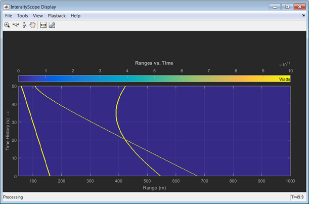
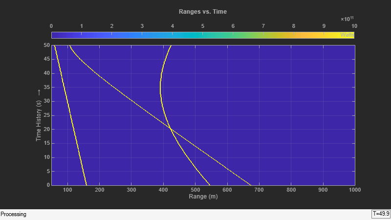
Use the phased.IntensityScope System object™ to display the intensities of the echoes of three moving targets as functions of range and time.
Create the Radar and Target System Objects
Set up the initial positions and velocities of the three targets. Use the phased.Platform System object to model radar and target motions. The radar is stationary while the targets undergo constant velocity motion. The simulation runs for 500 steps at 0.1 second increments, giving a total simulation time of 50 seconds.
nsteps = 500;
dt = .1;
timespan = nsteps*dt;
x1 = [60,0,0]';
x2 = [60,-80,40]';
x3 = [300,0,-300]';
v1 = [2,0,0]';
v2 = [10,5,6]';
v3 = [-10,2,-4]';
platform = phased.Platform([0,0,0]',[0,0,0]');
targets = phased.Platform([x1,x2,x3],[v1,v2,v3]);
Set Up Range Bins
Each echo is put into a range bin. The range bin resolution is 1 meter and the range is from 50 to 1000 meters.
rngres = 1.0;
rngmin = 50.0;
rngmax = 1000.0;
rngscan = [rngmin:rngres:rngmax];
Create the Gain Function
Define a range-dependent gain function to enhance the display of targets at larger ranges. The gain function amplifies the returned echo for visualization purposes only.
rangegain = @(rng)(1e12*rng^4);
Create the Intensity Scope
Set up the Intensity Scope using these properties.
Use the
XResolutionproperty to set the width of each scan line bin to the range resolution of 1 km.Use the
XOffsetproperty to set the value of the lowest range bin to the minimum range of 50 km.Use the
TimeResolutionproperty to set the value of the scan line time difference to 0.1 s.Use the
TimeSpanproperty to set the height of the display window to the time duration of the simulation.Use the
IntensityUnitsproperty to set the display units toWatts.
scope = phased.IntensityScope(Name="IntensityScope Display", ...
    Title="Ranges vs. Time",XLabel="Range (m)",XResolution=rngres,...
    XOffset=rngmin,TimeResolution=dt,TimeSpan=timespan, ...
    IntensityUnits="Watts",Position=[100,100,800,450]);
Run Simulation Loop
In this loop, move the targets at constant velocity using the
stepmethod of thephased.PlatformSystem object.Compute the target ranges using the
rangeanglefunction.Compute the target range bins by quantizing the range values in integer multiples of
rngres.Fill each target range bin and neighboring bins with a simulated radar intensity value.
Add the signal from each target to the scan line.
Call the
stepmethod of thephased.IntensityScopeSystem object to display the scan lines.
for k = 1:nsteps
    xradar = platform(dt);
    xtgts = targets(dt);
    [rngs] = rangeangle(xtgts,xradar);
    scanline = zeros(size(rngscan));

    rngindx = ceil((rngs(1) - rngmin)/rngres);
    scanline(rngindx + [-1:1]) = rangegain(rngs(1))/(rngs(1)^4);

    rngindx = ceil((rngs(2) - rngmin)/rngres);
    scanline(rngindx + [-1:1]) = rangegain(rngs(2))/(rngs(2)^4);

    rngindx = ceil((rngs(3) - rngmin)/rngres);
    scanline(rngindx + [-1:1]) = rangegain(rngs(3))/(rngs(3)^4);

    scope(scanline.');
    pause(.1);
end
Use the phased.IntensityScope System Object™ to display the detection output of a radar system simulation. The radar scenario contains a stationary single-element monostatic radar and three moving targets.
Set Radar Operating Parameters
Set the maximum range, peak power range resolution, operating frequency, transmitter gain, and target radar cross-section.
max_range = 5000;
range_res = 50;
fc = 10e9;
tx_gain = 20;
peak_power = 5500.0;
Choose the signal propagation speed to be the speed of light, and compute the signal wavelength corresponding to the operating frequency.
c = physconst("LightSpeed");
lambda = c/fc;
Compute the pulse bandwidth from the range resolution. Set the sampling rate, fs, to twice the pulse bandwidth. The noise bandwidth is also set to the pulse bandwidth. The radar integrates a number of pulses set by num_pulse_int. The duration of each pulse is the inverse of the pulse bandwidth.
pulse_bw = c/(2*range_res);
pulse_length = 1/pulse_bw;
fs = 2*pulse_bw;
noise_bw = pulse_bw;
num_pulse_int = 10;
Set the pulse repetition frequency to match the maximum range of the radar.
prf = c/(2*max_range);
Create System Objects for the Model
Choose a rectangular waveform.
waveform = phased.RectangularWaveform(PulseWidth=pulse_length, ...
    PRF=prf,SampleRate=fs);
Set the receiver amplifier characteristics.
amplifier = phased.ReceiverPreamp(Gain=20,NoiseFigure=0, ...
    SampleRate=fs,EnableInputPort=true,SeedSource="Property", ...
    Seed=2007);
transmitter = phased.Transmitter(Gain=tx_gain,PeakPower=peak_power, ...
    InUseOutputPort=true);
Specify the radar antenna as a single isotropic antenna.
antenna = phased.IsotropicAntennaElement(FrequencyRange=[5e9 15e9]);
Set up a monostatic radar platform.
radarplatform = phased.Platform(InitialPosition=[0; 0; 0], ...
    Velocity=[0; 0; 0]);
Set up the three target platforms using a single System object.
targetplatforms = phased.Platform(...
    InitialPosition=[2000.66 3532.63 3845.04; 0 0 0; 0 0 0], ...
    Velocity=[150 -150 0; 0 0 0; 0 0 0]);
Create the radiator and collector System objects.
radiator = phased.Radiator(Sensor=antenna,OperatingFrequency=fc);
collector = phased.Collector(Sensor=antenna,OperatingFrequency=fc);
Set up the three target RCS properties.
targets = phased.RadarTarget(MeanRCS=[1.6 2.2 1.05],OperatingFrequency=fc);
Create System object to model two-way freespace propagation.
channels= phased.FreeSpace(SampleRate=fs,TwoWayPropagation=true, ...
    OperatingFrequency=fc);
Define a matched filter.
MFcoef = getMatchedFilter(waveform);
mfilter = phased.MatchedFilter(Coefficients=MFcoef,GainOutputPort=true);
Create Range and Doppler Bins
Set up the fast-time grid. Fast time is the sampling time of the echoed pulse relative to the pulse transmission time. The range bins are the ranges corresponding to each bin of the fast time grid.
fast_time = unigrid(0,1/fs,1/prf,"[)");
range_bins = c*fast_time/2;
To compensate for range loss, create a time varying gain System Object.
gain = phased.TimeVaryingGain(RangeLoss=2*fspl(range_bins,lambda), ...
    ReferenceLoss=2*fspl(max_range,lambda));
Set up Doppler bins. Doppler bins are determined by the pulse repetition frequency. Create an FFT System object for Doppler processing.
DopplerFFTbins = 32;
DopplerRes = prf/DopplerFFTbins;
fft = dsp.FFT(FFTLengthSource="Property", ...
    FFTLength=DopplerFFTbins);
Create Data Cube
Set up a reduced data cube. Normally, a data cube has fast-time and slow-time dimensions and the number of sensors. Because the data cube has only one sensor, it is two-dimensional.
rx_pulses = zeros(numel(fast_time),num_pulse_int);
Create IntensityScope System Objects
Create two IntensityScope System objects, one for Doppler-time-intensity and the other for range-time-intensity.
dtiscope = phased.IntensityScope(Name="Doppler-Time Display", ...
    XLabel="Velocity (m/sec)", ...
    XResolution=dop2speed(DopplerRes,c/fc)/2, ...
    XOffset=dop2speed(-prf/2,c/fc)/2, ...
    TimeResolution=0.05,TimeSpan=5,IntensityUnits="Mag");
rtiscope = phased.IntensityScope(Name="Range-Time Display", ...
    XLabel="Range (m)", ...
    XResolution=c/(2*fs), ...
    TimeResolution=0.05,TimeSpan=5,IntensityUnits="Mag");
Run the Simulation Loop over Multiple Radar Transmissions
Transmit 2000 pulses. Coherently process groups of 10 pulses at a time.
For each pulse:
Update the radar position and velocity
radarplatformUpdate the target positions and velocities
targetplatformsCreate the pulses of a single wave train to be transmitted
transmitterCompute the ranges and angles of the targets with respect to the radar
Radiate the signals to the targets
radiatorPropagate the pulses to the target and back
channelsReflect the signals off the target
targetsReceive the signal
sCollectorAmplify the received signal
amplifierForm data cube
For each set of 10 pulses in the data cube:
Match filter each row (fast-time dimension) of the data cube.
Compute the Doppler shifts for each row (slow-time dimension) of the data cube.
pri = 1/prf;
nsteps = 200;
for k = 1:nsteps
    for m = 1:num_pulse_int
        [ant_pos,ant_vel] = radarplatform(pri);
        [tgt_pos,tgt_vel] = targetplatforms(pri);
        sig = waveform();
        [s,tx_status] = transmitter(sig);
        [~,tgt_ang] = rangeangle(tgt_pos,ant_pos);
        tsig = radiator(s,tgt_ang);
        tsig = channels(tsig,ant_pos,tgt_pos,ant_vel,tgt_vel);
        rsig = targets(tsig);
        rsig = collector(rsig,tgt_ang);
        rx_pulses(:,m) = amplifier(rsig,~(tx_status>0));
    end

    rx_pulses = mfilter(rx_pulses);
    MFdelay = size(MFcoef,1) - 1;
    rx_pulses = buffer(rx_pulses((MFdelay + 1):end), size(rx_pulses,1));
    rx_pulses = gain(rx_pulses);
    range = pulsint(rx_pulses,"noncoherent");
    rtiscope(range);
    dshift = fft(rx_pulses.');
    dshift = fftshift(abs(dshift),1);
    dtiscope(mean(dshift,2));
    radarplatform(.05);
    targetplatforms(.05);
end
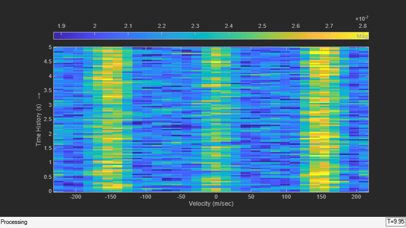
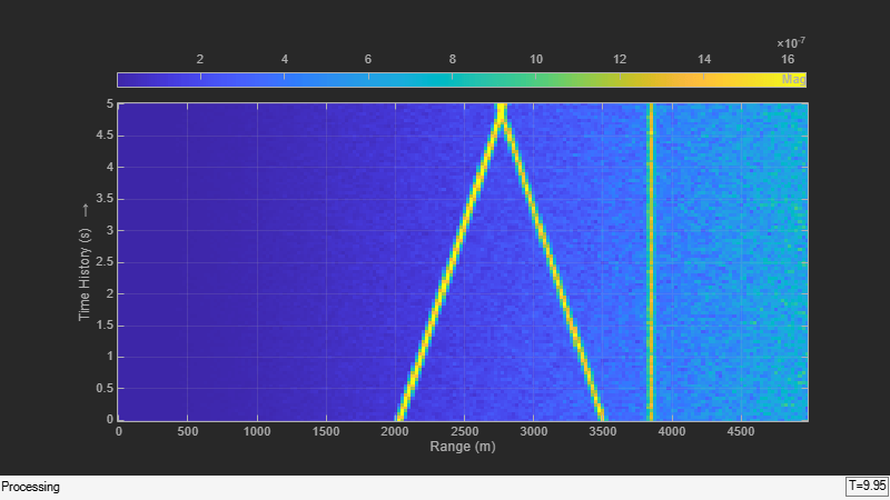
All of the targets lie on the x-axis. Two targets are moving along the x-axis and one is stationary. Because the radar is at the origin, you can read the target speed directly from the Doppler-Time Display window. The values agree with the specified velocities of -150, 150, and 0 m/sec.
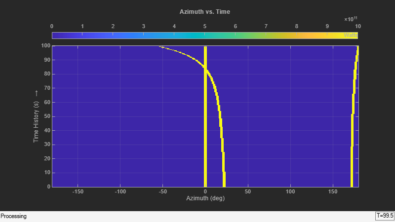
Use the phased.IntensityScope System object™ to display the angular motions of moving targets as functions of time. Each horizontal line (scan line) shows the strength of radar echoes at different azimuth angles. Azimuth space is divided into azimuth bins and each bin is filled with a simulated value depending upon the position of the targets.
Create Radar and Target System Objects
Set up the initial positions and velocities of the three targets. Use the phased.Platform System object to model radar and target motions. The radar is stationary while the targets undergo constant velocity motion. The simulation runs for 200 steps at 0.5 second intervals, giving a total simulation time of 100 seconds.
nsteps = 200;
dt = 0.5;
timespan = nsteps*dt;
x1 = [60,0,0]';
x2 = [60,-80,40]';
x3 = [300,0,-300]';
x3 = [-300,0,-300]';

v1 = [2,0,0]';
v2 = [10,5,6]';
v3 = [-10,2,-4]';
radarplatform = phased.Platform([0,0,0]',[0,0,0]');
targets = phased.Platform([x1,x2,x3],[v1,v2,v3]);
Set Up Azimuth Angle Bins
The signal for each echo is put into an angle bin and two adjacent bins. Bin resolution is 1 degree and the angle span is from −180 to 180 degrees.
angres = 1.0;
angmin = -180.0;
angmax = 180.0;
angscan = [angmin:angres:angmax];
na = length(angscan);
Range Gain Function
Define a range-dependent gain function to enhance the display of targets at larger ranges. The gain function amplifies the returned echo for visualization purposes only.
rangegain = @(rng)(1e12*rng^4);
Set Up Scope Viewer
The XResolution name-value pair specifies the width of each bin of the scan line. The XOffset sets the value of the lowest azimuth angle bin. The TimeResolution name-value pair specifies the time difference between scan lines. The TimeSpan name-value pair sets the height of the display window. A scan line is created with each call to the step method. Intensity units are amplitude units.
scope = phased.IntensityScope( ...
    Name="IntensityScope Display", ...
    Title="Azimuth vs. Time", ...
    XLabel="Azimuth (deg)", ...
    XResolution=angres,XOffset=angmin, ...
    TimeResolution=dt,TimeSpan=timespan, ...
    IntensityUnits="Watts", ...
    Position=[100,100,800,450]);
Update-Display Loop
In this loop, move the targets at constant velocity using the
stepmethod of thephased.PlatformSystem object.Compute the target ranges and azimuth angles using the
rangeanglefunction.Compute the azimuth angle bins by quantizing the azimuth angle values in integer multiples of
angres.Fill each target azimuth bin and neighboring bins with a simulated radar intensity value.
Call the
phased.IntensityScopestepmethod to display the scan line.
for k = 1:nsteps
    xradar = radarplatform(dt);
    xtgts = targets(dt);
    [rngs,angs] = rangeangle(xtgts,xradar);
    scanline = zeros(size(angscan));

    angindx = ceil((angs(1,1) - angmin)/angres) + 1;
    idx = angindx + [-1:1];
    idx(idx>na)=[];
    idx(idx<1)=[];
    scanline(idx) = rangegain(rngs(1))/(rngs(1)^4);

    angindx = ceil((angs(1,2) - angmin)/angres) + 1;
    idx = angindx + [-1:1];
    idx(idx>na)=[];
    idx(idx<1)=[];
    scanline(idx) = rangegain(rngs(2))/(rngs(2)^4);

    angindx = ceil((angs(1,3) - angmin)/angres) + 1;
    idx = angindx + [-1:1];
    idx(idx>na)=[];
    idx(idx<1)=[];
    scanline(idx) = rangegain(rngs(3))/(rngs(3)^4);
    scope(scanline.');
    pause(.1);
end